45 Recapitulation of Lecture 17

We touch on several points that were unclear or wrong in lecture 17. They have been corrected in the posted lecture notes, so we make only brief reference to them here.

45.1 Zero Knowledge Interactive Proof for Graph Isomorphism

Some of the difficulties stemmed from my failure to explicitly define the zero knowledge interactive proof (ZKIP) system (P,V ) for graph isomorphism (GI). The common input x is a pair of graphs (G₁,G₂) such that G₁G₂. The protocol in concise form is given in Figure 45.1

Prover P Verifier V 1. Random HG2. 2. Random σ {1,2}. 3. ψ: . Check H = ψ(Gσ). Figure 45.1: Interactive proof of graph isomorphism.

This answers the question of what P does with values σ ⁄{1,2} – it treats all such values as if σ = 1. It also explains the “normalization” of σ to the range {1,2} in the construction of the simulator M^*, for it seems to be necessary in order for the simulator to correctly mimic the behavior of the ⟨P,V ^*⟩(x).

45.2 Simulator for GI

The simulator M^* has to simulate ⟨P,V ^*⟩(x) for arbitrary polynomial time V ^* on common input x = (G₁,G₂) GI. It can’t directly simulate P since it must be polynomial time whereas P is not so restricted. Rather, it will guess V ^*’s message σ and choose H so that it can respond with a correct ψ. The simulator in concise form is given in Figure 45.2.

Simulator M* Arbitrary V * 1a. Random tape r for V *. 1b. Random τ {1,2}. 1c. Random permutation ψ on G2’s vertex set. 1d. H = ψ(Gτ). 2a. Run V *(x) with tapes x,r,H 2b. until σ = v*(x,r,H) produced. 3a. If σ = τ output (x,r,H,ψ). 3b. If σ≠τ output ⊥. Figure 45.2: Simulator for graph isomorphism prover.

Key issue in correctness proof of simulator is to show that σ and τ are independent. This is not a priori obvious since σ depends on H and H = ψ(G_τ) depends on τ. We want to show that

and similarly for τ = 2. That is, the a posteriori probability that τ = 1 is the same given H as it was a priori.

We use Bayes’ theorem to show this. (See section 41.) There are n! permutations ψ on a vertex set of size n. Therefore, Pr[ψ(G₁) = H] = Pr[ψ(G₂) = H] = . Since ψ is independent of τ, Pr[ψ(G_τ) = H] = . Clearly also Pr[τ = 1] = 1∕2. Plugging into Bayes’ theorem, we get

(1)

However, the conditional probability on the right side of equation 1 is easy to evaluate since the condition fixes the value of τ to be 1. Hence,

We conclude that

45.3 View distribution in the ZK proof for GI

The proof that viewP V^*(x) and m^*(x) are identically distributed is based on a few simple ideas. First of all, something stronger is proved: If we fix the random tape to a particular value r of V ^* and condition both viewP V ^*(x) and m^*(x) on the random tape being r, the resulting random variables, ν(x,r) and μ(x,r), respectively, are still identically distributed. This of course implies that the same holds when averaged over all possible r. Both of these variables range over 4-tuples (x,r,H,ψ). For simplicity, we also drop the first two components since they are always x and r. Hence, we consider the values of ν(x,r) and μ(x,r) to be pairs (H,ψ).

The fact that ν(x,r) and μ(x,r) are identically distributed follows from the claim that both are uniformly distributed over the set

Recall from Figure 45.2 that v^*(x,r,H) {1,2} is the value σ (after normalization) produced by V ^* in response to receiving message H, given that the common input is x and V ^*’s random tape is r. v^*() is an ordinary (not random) function since the machine V ^* becomes deterministic once its random tape has been fixed.

It is easy to show that the H-component of both ν(x,r) and μ(x,r) is uniformly distributed over the graphs isomorphic to G₂, given that x GI, since ψ is chosen uniformly at random from all permutations on the common vertex set of G₁ and G₂. Moreover, for each H, there is a unique permutation π such that (H,π) C_x,r. This is because the graph G_v^*(x,r,H)) is uniquely determined by x,r,H, and given two isomorphic graphs G′G′′, there is a unique isomorphism mapping one to the other. Let ψ₁ : G₁H and ψ₂ : G₂H. Then we can write

It remains to show that the random variables ν(x,r) and μ(x,r) both range over C_x,r.

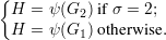
Let ν(x,r) = (H,ψ). ψ is the value returned by P in step 3. (See Figure 45.1.) This is indeed ψ_σ, where σ = v^*(x,r,H) is the value returned by V ^* in step 2. Hence, ν(x,r) C_x,r.

Let μ(x,r) = (H,ψ). Since we are assuming the simulator does not output ⊥, we have that σ = τ, where σ = v^*(x,r,H) is the value produced by the simulation of V ^* starting from x,r,H and τ is the value computed by the simulator in step 1b. (See Figure 45.1.) ψ is chosen in step 1c of the simulator to be a random permutation on G₂’s vertex set and is placed in the output tuple in step 3a. H = ψ(G_τ) is computed in step 1d, so ψ = ψ_τ = ψ_σ. Hence, μ(x,r) C_x,r.

We conclude that ν(x,r) and μ(x,r) are identically distributed, which concludes the proof that (P,V ) is a ZKIP for GI.

46 Sequential Composition of Zero Knowledge Proofs

When we use zero knowledge proofs, we will often repeat them many times to make the error probability sufficiently small. This raises the issue of whether the repeated protocol is zero knowledge even if a single instance is. The problem is that with several repetitions, an adversary V ^* is gaining data from all of the previous ones. Even though one repetition might not give the adversary additional computational power, it doesn’t follow a priori that the same will be true for multiple repetitions. It turns out that zero knowledge is closed under such repetitions, but we first need a stronger version of zero knowledge based on interactive proofs with auxiliary inputs.

46.1 Zero Knowledge with Respect to Auxiliary Inputs

Let (P,V ) be an interactive proof system with auxiliary inputs for a language L. (See section  42.) We provide both prover and verifier with private auxiliary input tapes. Recall that ⟨P(y),V (z)⟩(x) is V ’s output when the common input is x, P has private input y, and V has private input z. (P,V ) satisfy the completeness and soundness conditions of section 42.

For each x L, let P_L(x) be the set of strings y that satisfy the completeness condition. That is, P_L(x) is the set of y such that for all z,

We say that (P,V ) is zero knowledge with respect to auxiliary inputs if for every probabilistic polynomial-time interactive Turing machine V ^*, there exists a probabilistic algorithm M^*(x,y) that runs in time polynomial in |x| called the simulator. For all x L and y P_L(x), the output distribution of M^*(x,y) must be computationally indistinguishable from the output distribution of ⟨P(y),V ^*(z)⟩(x).¹ Equivalently, this requirement says that for every probabilistic algorithm D with running time polynomial in the length of its first input, for every polynomial p(⋅), and for all sufficiently long x L, all y P_L(x), and all z {0,1}^*, it holds that

46.2 Closure Under Sequential Composition

The goal of this section is to show that if (P,V ) is a zero knowledge interactive proof system with respect to auxiliary inputs for a language L, then the sequential composition (repetition) of polynomially many copies of P is also zero knowledge with respect to auxiliary inputs. That is, if one round of P does not leak any useful knowledge to an adversary V ^*, then still no useful knowledge is leaked even if V ^* is permitted multiple rounds of interaction with P . Formally, we need to construct a simulator for the computation⟨P,V ^*(z)⟩(x), where V ^* is a polynomial-time machine with auxiliary input that can interact with P multiple times.

We only briefly survey this topic, referring the reader to sections 4.3.3 and 4.3.4 of the textbook for further details.

Here’s the overall plan. One starts with an interactive proof system (P,V ) for L with auxiliary inputs. Now consider the interactive protocol (P,V ^*), where V ^* may interact with P for a polynomial number of rounds. A round from P ’s point of view is a complete run of its specified protocol. In each round, P starts in its prescribed initial state with the common input on its input tape and a fresh random string on its random tape. V ^* however views P as a server that can be invoked polynomially many times. It does not start over on each round but rather continues its computation from the previous round.

The simulator M^* for V ^* is constructed in several stages:

1. We construct a machine V ^** that performs one round of interaction with P . It takes as input a configuration of V ^* and simulates the execution of V ^* beginning from that configuration until V ^* completes one round of interaction with P . It then outputs the current configuration of V ^* and halts. If we chain together polynomially many executions of V ^**, we get the same effect as running V ^*. The chaining simply means copying the output tape of V ^** back onto the auxiliary input tape and running V ^** again.

   I’ve glossed over a lot of details, such as how V ^** knows when the end of a round is, how to pass the real auxiliary input of V ^* to V ^**, and how to produce the final output of V ^**, but this is the rough idea.

2. Next, we construct the simulator M^** for V ^**. This is possible since we are assuming that P is zero knowledge, and V ^** is just some polynomial time auxiliary input Turing machine.
3. Now, we construct the simulator M^*. It just runs a loop, calling M^** repeatedly.
4. We use a hybrid argument to show that ⟨P(y),V ^*(z)⟩(x) is computationally indistinguishable from M^*(x,z) for all y P_L(x). The argument looks at the developing view stage by stage and argues if the whole views are distinguishable, then there must be some stage where the view first became distinguishable. From that, one derives a contradiction to the assumption that P is zero knowledge.

This is pretty sparse, but it should give some general idea at least of the structure of the proof.