March 23 - More Learning

from learning import *
from notebook import *

Iris in Wonderland

Setosa

Versicolor

Virginia

Fisher's Iris data set

MACHINE LEARNING OVERVIEW

In this notebook, we learn about agents that can improve their behavior through diligent study of their own experiences.

An agent is learning if it improves its performance on future tasks after making observations about the world.

There are three types of feedback that determine the three main types of learning:

• Supervised Learning:

In Supervised Learning the agent observes some example input-output pairs and learns a function that maps from input to output.

Example: Let's think of an agent to classify images containing cats or dogs. If we provide an image containing a cat or a dog, this agent should output a string "cat" or "dog" for that particular image. To teach this agent, we will give a lot of input-output pairs like {cat image-"cat"}, {dog image-"dog"} to the agent. The agent then learns a function that maps from an input image to one of those strings.

• Unsupervised Learning:

In Unsupervised Learning the agent learns patterns in the input even though no explicit feedback is supplied. The most common type is clustering: detecting potential useful clusters of input examples.

Example: A taxi agent would develop a concept of good traffic days and bad traffic days without ever being given labeled examples.

• Reinforcement Learning:

In Reinforcement Learning the agent learns from a series of reinforcements—rewards or punishments.

Example: Let's talk about an agent to play the popular Atari game—Pong. We will reward a point for every correct move and deduct a point for every wrong move from the agent. Eventually, the agent will figure out its actions prior to reinforcement were most responsible for it.

DATASETS

For the following tutorials we will use a range of datasets, to better showcase the strengths and weaknesses of the algorithms. The datasests are the following:

• Fisher's Iris: Each item represents a flower, with four measurements: the length and the width of the sepals and petals. Each item/flower is categorized into one of three species: Setosa, Versicolor and Virginica.

• Zoo: The dataset holds different animals and their classification as "mammal", "fish", etc. The new animal we want to classify has the following measurements: 1, 0, 0, 1, 0, 0, 0, 1, 1, 1, 0, 0, 4, 1, 0, 1 (don't concern yourself with what the measurements mean).

To make using the datasets easier, we have written a class, DataSet, in learning.py. The tutorials found here make use of this class.

Let's have a look at how it works before we get started with the algorithms.

Intro

A lot of the datasets we will work with are .csv files (although other formats are supported too). We have a collection of sample datasets ready to use on aima-data. Two examples are the datasets mentioned above (iris.csv and zoo.csv). You can find plenty datasets online, and a good repository of such datasets is UCI Machine Learning Repository.

In such files, each line corresponds to one item/measurement. Each individual value in a line represents a feature and usually there is a value denoting the class of the item.

You can find the code for the dataset here:

Importing a Dataset

Importing from aima-data

Datasets uploaded on aima-data can be imported with the following line:

iris = DataSet(name="iris")

When importing a dataset, we can specify to exclude an attribute (for example, at index 1) by setting the parameter exclude to the attribute index or name.

iris2 = DataSet(name="iris")

iris2.remove_examples("virginica")
print(iris2.values[iris2.target])

['versicolor', 'setosa']

len(iris2.examples)

100

RANDOM FOREST LEARNER

Overview

Image via src

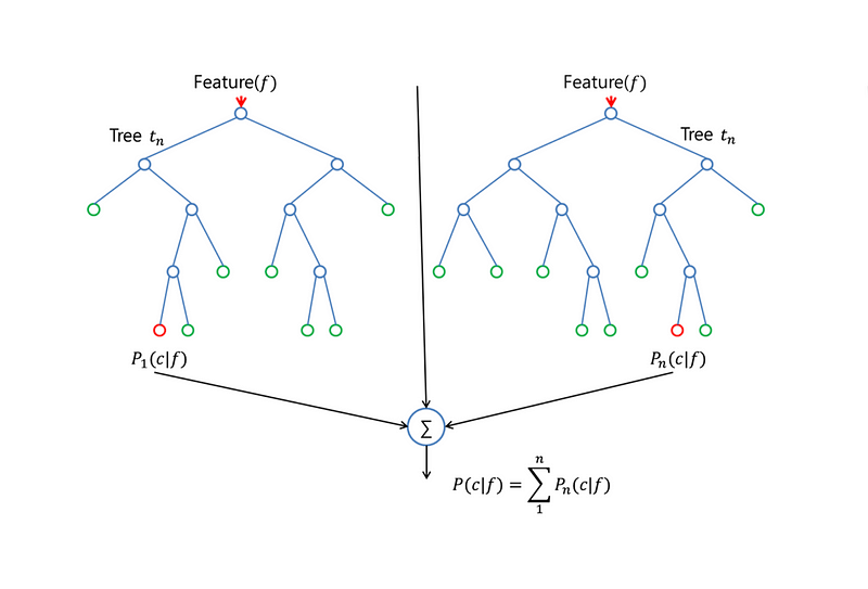
Random Forest

As the name of the algorithm and image above suggest, this algorithm creates the forest with a number of trees. The greater number of trees makes the forest robust. In the same way in random forest algorithm, the higher the number of trees in the forest, the higher is the accuray result. The main difference between Random Forest and Decision trees is that, finding the root node and splitting the feature nodes will be random.

Let's see how Rnadom Forest Algorithm work :

Random Forest Algorithm works in two steps, first is the creation of random forest and then the prediction. Let's first see the creation :

The first step in creation is to randomly select 'm' features out of total 'n' features. From these 'm' features calculate the node d using the best split point and then split the node into further nodes using best split. Repeat these steps until 'i' number of nodes are reached. Repeat the entire whole process to build the forest.

Now, let's see how the prediction works Take the test features and predict the outcome for each randomly created decision tree. Calculate the votes for each prediction and the prediction which gets the highest votes would be the final prediction.

Implementation

Below mentioned is the implementation of Random Forest Algorithm.

psource(RandomForest)

def RandomForest(dataset, n=5):
    """An ensemble of Decision Trees trained using bagging and feature bagging."""

    def data_bagging(dataset, m=0):
        """Sample m examples with replacement"""
        n = len(dataset.examples)
        return weighted_sample_with_replacement(m or n, dataset.examples, [1]*n)

    def feature_bagging(dataset, p=0.7):
        """Feature bagging with probability p to retain an attribute"""
        inputs = [i for i in dataset.inputs if probability(p)]
        return inputs or dataset.inputs

    def predict(example):
        print([predictor(example) for predictor in predictors])
        return mode(predictor(example) for predictor in predictors)

    predictors = [DecisionTreeLearner(DataSet(examples=data_bagging(dataset),
                                              attrs=dataset.attrs,
                                              attrnames=dataset.attrnames,
                                              target=dataset.target,
                                              inputs=feature_bagging(dataset))) for _ in range(n)]

    return predict

This algorithm creates an ensemble of decision trees using bagging and feature bagging. It takes 'm' examples randomly from the total number of examples and then perform feature bagging with probability p to retain an attribute. All the predictors are predicted from the DecisionTreeLearner and then a final prediction is made.

Example

We will now use the Random Forest to classify a sample with values: 5.1, 3.0, 1.1, 0.1.

iris = DataSet(name="iris")

RFL = RandomForest(iris, n=5)
print(RFL([5.1, 3.0, 1.1, 0.1]))

['setosa', 'setosa', 'versicolor', 'setosa', 'setosa']
setosa

RFL = RandomForest(iris, n=3)
print(RFL([5.1, 3.0, 1.1, 0.1]))

['setosa', 'setosa', 'setosa']
setosa

As expected, the Random Forest classifies the sample as "setosa".

weighted_sample_with_replacement(5, iris.examples, [1]*5)

[[5.1, 3.5, 1.4, 0.2, 'setosa'],
 [5.0, 3.6, 1.4, 0.2, 'setosa'],
 [5.1, 3.5, 1.4, 0.2, 'setosa'],
 [5.1, 3.5, 1.4, 0.2, 'setosa'],
 [5.1, 3.5, 1.4, 0.2, 'setosa']]

psource(weighted_sample_with_replacement)

def weighted_sample_with_replacement(n, seq, weights):
    """Pick n samples from seq at random, with replacement, with the
    probability of each element in proportion to its corresponding
    weight."""
    sample = weighted_sampler(seq, weights)

    return [sample() for _ in range(n)]

NAIVE BAYES LEARNER

Overview

Theory of Probabilities

The Naive Bayes algorithm is a probabilistic classifier, making use of Bayes' Theorem. The theorem states that the conditional probability of A given B equals the conditional probability of B given A multiplied by the probability of A, divided by the probability of B.

$$P(A|B) = \dfrac{P(B|A)*P(A)}{P(B)}$$

From the theory of Probabilities we have the Multiplication Rule, if the events X are independent the following is true:

$$P(X_{1} \cap X_{2} \cap ... \cap X_{n}) = P(X_{1})*P(X_{2})*...*P(X_{n})$$

For conditional probabilities this becomes:

$$P(X_{1}, X_{2}, ..., X_{n}|Y) = P(X_{1}|Y)*P(X_{2}|Y)*...*P(X_{n}|Y)$$

Classifying an Item

How can we use the above to classify an item though?

We have a dataset with a set of classes (C) and we want to classify an item with a set of features (F). Essentially what we want to do is predict the class of an item given the features.

For a specific class, Class, we will find the conditional probability given the item features:

$$P(Class|F) = \dfrac{P(F|Class)*P(Class)}{P(F)}$$

We will do this for every class and we will pick the maximum. This will be the class the item is classified in.

The features though are a vector with many elements. We need to break the probabilities up using the multiplication rule. Thus the above equation becomes:

$$P(Class|F) = \dfrac{P(Class)*P(F_{1}|Class)*P(F_{2}|Class)*...*P(F_{n}|Class)}{P(F_{1})*P(F_{2})*...*P(F_{n})}$$

The calculation of the conditional probability then depends on the calculation of the following:

a) The probability of Class in the dataset.

b) The conditional probability of each feature occurring in an item classified in Class.

c) The probabilities of each individual feature.

For a), we will count how many times Class occurs in the dataset (aka how many items are classified in a particular class).

For b), if the feature values are discrete ('Blue', '3', 'Tall', etc.), we will count how many times a feature value occurs in items of each class. If the feature values are not discrete, we will go a different route. We will use a distribution function to calculate the probability of values for a given class and feature. If we know the distribution function of the dataset, then great, we will use it to compute the probabilities. If we don't know the function, we can assume the dataset follows the normal (Gaussian) distribution without much loss of accuracy. In fact, it can be proven that any distribution tends to the Gaussian the larger the population gets (see Central Limit Theorem).

NOTE: If the values are continuous but use the discrete approach, there might be issues if we are not lucky. For one, if we have two values, '5.0 and 5.1', with the discrete approach they will be two completely different values, despite being so close. Second, if we are trying to classify an item with a feature value of '5.15', if the value does not appear for the feature, its probability will be 0. This might lead to misclassification. Generally, the continuous approach is more accurate and more useful, despite the overhead of calculating the distribution function.

The last one, c), is tricky. If feature values are discrete, we can count how many times they occur in the dataset. But what if the feature values are continuous? Imagine a dataset with a height feature. Is it worth it to count how many times each value occurs? Most of the time it is not, since there can be miscellaneous differences in the values (for example, 1.7 meters and 1.700001 meters are practically equal, but they count as different values).

So as we cannot calculate the feature value probabilities, what are we going to do?

Let's take a step back and rethink exactly what we are doing. We are essentially comparing conditional probabilities of all the classes. For two classes, A and B, we want to know which one is greater:

$$\dfrac{P(F|A)*P(A)}{P(F)} vs. \dfrac{P(F|B)*P(B)}{P(F)}$$

Wait, P(F) is the same for both the classes! In fact, it is the same for every combination of classes. That is because P(F) does not depend on a class, thus being independent of the classes.

So, for c), we actually don't need to calculate it at all.

Wrapping It Up

Classifying an item to a class then becomes a matter of calculating the conditional probabilities of feature values and the probabilities of classes. This is something very desirable and computationally delicious.

Remember though that all the above are true because we made the assumption that the features are independent. In most real-world cases that is not true though. Is that an issue here? Fret not, for the the algorithm is very efficient even with that assumption. That is why the algorithm is called Naive Bayes Classifier. We (naively) assume that the features are independent to make computations easier.

Implementation

The implementation of the Naive Bayes Classifier is split in two; Learning and Simple. The learning classifier takes as input a dataset and learns the needed distributions from that. It is itself split into two, for discrete and continuous features. The simple classifier takes as input not a dataset, but already calculated distributions (a dictionary of CountingProbDist objects).

Discrete

The implementation for discrete values counts how many times each feature value occurs for each class, and how many times each class occurs. The results are stored in a CountinProbDist object.

With the below code you can see the probabilities of the class "Setosa" appearing in the dataset and the probability of the first feature (at index 0) of the same class having a value of 5. Notice that the second probability is relatively small, even though if we observe the dataset we will find that a lot of values are around 5. The issue arises because the features in the Iris dataset are continuous, and we are assuming they are discrete. If the features were discrete (for example, "Tall", "3", etc.) this probably wouldn't have been the case and we would see a much nicer probability distribution.

psource(CountingProbDist)

class CountingProbDist:
    """A probability distribution formed by observing and counting examples.
    If p is an instance of this class and o is an observed value, then
    there are 3 main operations:
    p.add(o) increments the count for observation o by 1.
    p.sample() returns a random element from the distribution.
    p[o] returns the probability for o (as in a regular ProbDist)."""

    def __init__(self, observations=None, default=0):
        """Create a distribution, and optionally add in some observations.
        By default this is an unsmoothed distribution, but saying default=1,
        for example, gives you add-one smoothing."""
        if observations is None:
            observations = []
        self.dictionary = {}
        self.n_obs = 0
        self.default = default
        self.sampler = None

        for o in observations:
            self.add(o)

    def add(self, o):
        """Add an observation o to the distribution."""
        self.smooth_for(o)
        self.dictionary[o] += 1
        self.n_obs += 1
        self.sampler = None

    def smooth_for(self, o):
        """Include o among the possible observations, whether or not
        it's been observed yet."""
        if o not in self.dictionary:
            self.dictionary[o] = self.default
            self.n_obs += self.default
            self.sampler = None

    def __getitem__(self, item):
        """Return an estimate of the probability of item."""
        self.smooth_for(item)
        return self.dictionary[item] / self.n_obs

    # (top() and sample() are not used in this module, but elsewhere.)

    def top(self, n):
        """Return (count, obs) tuples for the n most frequent observations."""
        return heapq.nlargest(n, [(v, k) for (k, v) in self.dictionary.items()])

    def sample(self):
        """Return a random sample from the distribution."""
        if self.sampler is None:
            self.sampler = weighted_sampler(list(self.dictionary.keys()),
                                            list(self.dictionary.values()))
        return self.sampler()

Statistical Learning

Chapter 20, page 802

There are five types of bags of candies. Each bag has 100 pieces, individually wrapped. One bag has all cherry (yum). One bag has all lime (yuck). The wrapping paper is identical and opaque.

Three other bags have a mixture: (75 cherry, 25 lime), (50 each), (25 cherry, 75 lime).

The bags themselves are not evenly distributed. 10% are all cherry and 10% are all lime. 40% are 50/50, and 20% are either 25% lime or 25% cherry.

If I give you a bag at random, you can randomly sample one candy at a time (and then rewrap it put it back in the bag).

You pick a random bag and start sampling. If you select one lime candy, what is the most likely bag? What you pick two in row? Three in row? Four in a row?

We can use the CountingProbDist() to model this problem.

h1 = CountingProbDist('c'*100)
h2 = CountingProbDist('c'*75+'l'*25)
h3 = CountingProbDist('c'*50+'l'*50)
h4 = CountingProbDist('c'*25+'l'*75)
h5 = CountingProbDist('l'*100)
dist = {('h1', 0.1): h1, ('h2', 0.2): h2, ('h3', 0.4): h3, 
        ('h4', 0.2): h4, ('h5', 0.1): h5}
nBS = NaiveBayesLearner(dist, simple=True)

See Figure 20.1 on page 804

print (nBS('l'))
print (nBS('ll'))
print (nBS('lll'))
print (nBS('llll'))

h3
h4
h5
h5

Back to the flowers

It is spring, you know.

dataset = iris

target_vals = dataset.values[dataset.target]
target_dist = CountingProbDist(target_vals)
attr_dists = {(gv, attr): CountingProbDist(dataset.values[attr])
              for gv in target_vals
              for attr in dataset.inputs}
for example in dataset.examples:
        targetval = example[dataset.target]
        target_dist.add(targetval)
        for attr in dataset.inputs:
            attr_dists[targetval, attr].add(example[attr])


print(target_dist['setosa'])
print(attr_dists['setosa', 0][5.0])

0.3333333333333333
0.10588235294117647

target_dist

<learning.CountingProbDist at 0x7f44ae250c50>

First we found the different values for the classes (called targets here) and calculated their distribution. Next we initialized a dictionary of CountingProbDist objects, one for each class and feature. Finally, we iterated through the examples in the dataset and calculated the needed probabilites.

Having calculated the different probabilities, we will move on to the predicting function. It will receive as input an item and output the most likely class. Using the above formula, it will multiply the probability of the class appearing, with the probability of each feature value appearing in the class. It will return the max result.

def predict(example):
    def class_probability(targetval):
        return (target_dist[targetval] *
                product(attr_dists[targetval, attr][example[attr]]
                        for attr in dataset.inputs))
    return argmax(target_vals, key=class_probability)


print(predict([5, 3, 1, 0.1]))

setosa

You can view the complete code by executing the next line:

psource(NaiveBayesDiscrete)

def NaiveBayesDiscrete(dataset):
    """Just count how many times each value of each input attribute
    occurs, conditional on the target value. Count the different
    target values too."""

    target_vals = dataset.values[dataset.target]
    target_dist = CountingProbDist(target_vals)
    attr_dists = {(gv, attr): CountingProbDist(dataset.values[attr])
                  for gv in target_vals
                  for attr in dataset.inputs}
    for example in dataset.examples:
        targetval = example[dataset.target]
        target_dist.add(targetval)
        for attr in dataset.inputs:
            attr_dists[targetval, attr].add(example[attr])

    def predict(example):
        """Predict the target value for example. Consider each possible value,
        and pick the most likely by looking at each attribute independently."""
        def class_probability(targetval):
            return (target_dist[targetval] *
                    product(attr_dists[targetval, attr][example[attr]]
                            for attr in dataset.inputs))
        return argmax(target_vals, key=class_probability)

    return predict

Continuous

In the implementation we use the Gaussian/Normal distribution function. To make it work, we need to find the means and standard deviations of features for each class. We make use of the find_means_and_deviations Dataset function. On top of that, we will also calculate the class probabilities as we did with the Discrete approach.

means, deviations = dataset.find_means_and_deviations()

target_vals = dataset.values[dataset.target]
target_dist = CountingProbDist(target_vals)


print(means["setosa"])
print(deviations["setosa"])

print(means["versicolor"])
print(deviations["versicolor"])

[5.006, 3.418, 1.464, 0.244]
[0.3524896872134513, 0.38102439795469095, 0.17351115943644546, 0.10720950308167838]
[5.936, 2.77, 4.26, 1.326]
[0.5161711470638634, 0.3137983233784114, 0.46991097723995795, 0.19775268000454405]

You can see the means of the features for the "Setosa" class and the deviations for "Versicolor".

The prediction function will work similarly to the Discrete algorithm. It will multiply the probability of the class occurring with the conditional probabilities of the feature values for the class.

Since we are using the Gaussian distribution, we will input the value for each feature into the Gaussian function, together with the mean and deviation of the feature. This will return the probability of the particular feature value for the given class. We will repeat for each class and pick the max value.

def predict(example):
    def class_probability(targetval):
        prob = target_dist[targetval]
        for attr in dataset.inputs:
            prob *= gaussian(means[targetval][attr], deviations[targetval][attr], example[attr])
        return prob

    return argmax(target_vals, key=class_probability)


print(predict([5, 3, 1, 0.1]))

setosa

The complete code of the continuous algorithm:

psource(NaiveBayesContinuous)

def NaiveBayesContinuous(dataset):
    """Count how many times each target value occurs.
    Also, find the means and deviations of input attribute values for each target value."""
    means, deviations = dataset.find_means_and_deviations()

    target_vals = dataset.values[dataset.target]
    target_dist = CountingProbDist(target_vals)

    def predict(example):
        """Predict the target value for example. Consider each possible value,
        and pick the most likely by looking at each attribute independently."""
        def class_probability(targetval):
            prob = target_dist[targetval]
            for attr in dataset.inputs:
                prob *= gaussian(means[targetval][attr], deviations[targetval][attr], example[attr])
            return prob

        return argmax(target_vals, key=class_probability)

    return predict

Simple

The simple classifier (chosen with the argument simple) does not learn from a dataset, instead it takes as input a dictionary of already calculated CountingProbDist objects and returns a predictor function. The dictionary is in the following form: (Class Name, Class Probability): CountingProbDist Object.

Each class has its own probability distribution. The classifier given a list of features calculates the probability of the input for each class and returns the max. The only pre-processing work is to create dictionaries for the distribution of classes (named targets) and attributes/features.

The complete code for the simple classifier:

psource(NaiveBayesSimple)

def NaiveBayesSimple(distribution):
    """A simple naive bayes classifier that takes as input a dictionary of
    CountingProbDist objects and classifies items according to these distributions.
    The input dictionary is in the following form:
        (ClassName, ClassProb): CountingProbDist"""
    target_dist = {c_name: prob for c_name, prob in distribution.keys()}
    attr_dists = {c_name: count_prob for (c_name, _), count_prob in distribution.items()}

    def predict(example):
        """Predict the target value for example. Calculate probabilities for each
        class and pick the max."""
        def class_probability(targetval):
            attr_dist = attr_dists[targetval]
            return target_dist[targetval] * product(attr_dist[a] for a in example)

        return argmax(target_dist.keys(), key=class_probability)

    return predict

This classifier is useful when you already have calculated the distributions and you need to predict future items.

Examples

We will now use the Naive Bayes Classifier (Discrete and Continuous) to classify items:

nBD = NaiveBayesLearner(iris, continuous=False)
print("Discrete Classifier")
print(nBD([5, 3, 1, 0.1]))
print(nBD([6, 5, 3, 1.5]))
print(nBD([7, 3, 6.5, 2]))


nBC = NaiveBayesLearner(iris, continuous=True)
print("\nContinuous Classifier")
print(nBC([5, 3, 1, 0.1]))
print(nBC([6, 5, 3, 1.5]))
print(nBC([7, 3, 6.5, 2]))

Discrete Classifier
setosa
versicolor
versicolor

Continuous Classifier
setosa
versicolor
virginica

Notice how the Discrete Classifier misclassified the second item, while the Continuous one had no problem.

Let's now take a look at the simple classifier. First we will come up with a sample problem to solve. Say we are given three bags. Each bag contains three letters ('a', 'b' and 'c') of different quantities. We are given a string of letters and we are tasked with finding from which bag the string of letters came.

Since we know the probability distribution of the letters for each bag, we can use the naive bayes classifier to make our prediction.

bag1 = 'a'*50 + 'b'*30 + 'c'*15
dist1 = CountingProbDist(bag1)
bag2 = 'a'*30 + 'b'*45 + 'c'*20
dist2 = CountingProbDist(bag2)
bag3 = 'a'*20 + 'b'*20 + 'c'*35
dist3 = CountingProbDist(bag3)

Now that we have the CountingProbDist objects for each bag/class, we will create the dictionary. We assume that it is equally probable that we will pick from any bag.

dist = {('First', 0.5): dist1, ('Second', 0.3): dist2, ('Third', 0.2): dist3}
nBS = NaiveBayesLearner(dist, simple=True)

Now we can start making predictions:

print(nBS('aab'))        # We can handle strings
print(nBS(['b', 'b']))   # And lists!
print(nBS('ccbcc'))

First
Second
Third

The results make intuitive sense. The first bag has a high amount of 'a's, the second has a high amount of 'b's and the third has a high amount of 'c's. The classifier seems to confirm this intuition.

Note that the simple classifier doesn't distinguish between discrete and continuous values. It just takes whatever it is given. Also, the simple option on the NaiveBayesLearner overrides the continuous argument. NaiveBayesLearner(d, simple=True, continuous=False) just creates a simple classifier.

PERCEPTRON CLASSIFIER

Overview

The Perceptron is a linear classifier. It works the same way as a neural network with no hidden layers (just input and output). First it trains its weights given a dataset and then it can classify a new item by running it through the network.

Its input layer consists of the the item features, while the output layer consists of nodes (also called neurons). Each node in the output layer has n synapses (for every item feature), each with its own weight. Then, the nodes find the dot product of the item features and the synapse weights. These values then pass through an activation function (usually a sigmoid). Finally, we pick the largest of the values and we return its index.

Note that in classification problems each node represents a class. The final classification is the class/node with the max output value.

Below you can see a single node/neuron in the outer layer. With f we denote the item features, with w the synapse weights, then inside the node we have the dot product and the activation function, g.

Implementation

First, we train (calculate) the weights given a dataset, using the BackPropagationLearner function of learning.py. We then return a function, predict, which we will use in the future to classify a new item. The function computes the (algebraic) dot product of the item with the calculated weights for each node in the outer layer. Then it picks the greatest value and classifies the item in the corresponding class.

psource(PerceptronLearner)

def PerceptronLearner(dataset, learning_rate=0.01, epochs=100):
    """Logistic Regression, NO hidden layer"""
    i_units = len(dataset.inputs)
    o_units = len(dataset.values[dataset.target])
    hidden_layer_sizes = []
    raw_net = network(i_units, hidden_layer_sizes, o_units)
    learned_net = BackPropagationLearner(dataset, raw_net, learning_rate, epochs)

    def predict(example):
        o_nodes = learned_net[1]

        # Forward pass
        for node in o_nodes:
            in_val = dotproduct(example, node.weights)
            node.value = node.activation(in_val)

        # Hypothesis
        return find_max_node(o_nodes)

    return predict

Note that the Perceptron is a one-layer neural network, without any hidden layers. So, in BackPropagationLearner, we will pass no hidden layers. From that function we get our network, which is just one layer, with the weights calculated.

That function predict passes the input/example through the network, calculating the dot product of the input and the weights for each node and returns the class with the max dot product.

Example

We will train the Perceptron on the iris dataset. Because though the BackPropagationLearner works with integer indexes and not strings, we need to convert class names to integers. Then, we will try and classify the item/flower with measurements of 5, 3, 1, 0.1.

iris = DataSet(name="iris")
iris.classes_to_numbers()

perceptron = PerceptronLearner(iris)
print(perceptron([5, 3, 1, 0.1]))

0

The correct output is 0, which means the item belongs in the first class, "setosa". Note that the Perceptron algorithm is not perfect and may produce false classifications.

LINEAR LEARNER

Overview

Linear Learner is a model that assumes a linear relationship between the input variables x and the single output variable y. More specifically, that y can be calculated from a linear combination of the input variables x. Linear learner is a quite simple model as the representation of this model is a linear equation.

The linear equation assigns one scaler factor to each input value or column, called a coefficients or weights. One additional coefficient is also added, giving additional degree of freedom and is often called the intercept or the bias coefficient.
For example : y = ax1 + bx2 + c .

Implementation

Below mentioned is the implementation of Linear Learner.

psource(LinearLearner)

def LinearLearner(dataset, learning_rate=0.01, epochs=100):
    """Define with learner = LinearLearner(data); infer with learner(x)."""
    idx_i = dataset.inputs
    idx_t = dataset.target  # As of now, dataset.target gives only one index.
    examples = dataset.examples
    num_examples = len(examples)

    # X transpose
    X_col = [dataset.values[i] for i in idx_i]  # vertical columns of X

    # Add dummy
    ones = [1 for _ in range(len(examples))]
    X_col = [ones] + X_col

    # Initialize random weigts
    num_weights = len(idx_i) + 1
    w = random_weights(min_value=-0.5, max_value=0.5, num_weights=num_weights)

    for epoch in range(epochs):
        err = []
        # Pass over all examples
        for example in examples:
            x = [1] + example
            y = dotproduct(w, x)
            t = example[idx_t]
            err.append(t - y)

        # update weights
        for i in range(len(w)):
            w[i] = w[i] + learning_rate * (dotproduct(err, X_col[i]) / num_examples)

    def predict(example):
        x = [1] + example
        return dotproduct(w, x)
    return predict

This algorithm first assigns some random weights to the input variables and then based on the error calculated updates the weight for each variable. Finally the prediction is made with the updated weights.

Implementation

We will now use the Linear Learner to classify a sample with values: 5.1, 3.0, 1.1, 0.1.

iris = DataSet(name="iris")
iris.classes_to_numbers()

linear_learner = LinearLearner(iris)
print(linear_learner([5, 3, 1, 0.1]))

0.38413573818785207

ENSEMBLE LEARNER

Overview

Ensemble Learning improves the performance of our model by combining several learners. It improvise the stability and predictive power of the model. Ensemble methods are meta-algorithms that combine several machine learning techniques into one predictive model in order to decrease variance, bias, or improve predictions.

Some commonly used Ensemble Learning techniques are :

1. Bagging : Bagging tries to implement similar learners on small sample populations and then takes a mean of all the predictions. It helps us to reduce variance error.

2. Boosting : Boosting is an iterative technique which adjust the weight of an observation based on the last classification. If an observation was classified incorrectly, it tries to increase the weight of this observation and vice versa. It helps us to reduce bias error.

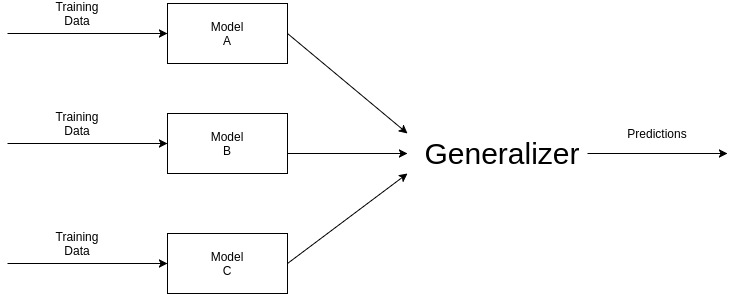
3. Stacking : This is a very interesting way of combining models. Here we use a learner to combine output from different learners. It can either decrease bias or variance error depending on the learners we use.

Implementation

Below mentioned is the implementation of Ensemble Learner.

psource(EnsembleLearner)

def EnsembleLearner(learners):
    """Given a list of learning algorithms, have them vote."""
    def train(dataset):
        predictors = [learner(dataset) for learner in learners]

        def predict(example):
            return mode(predictor(example) for predictor in predictors)
        return predict
    return train

This algorithm takes input as a list of learning algorithms, have them vote and then finally returns the predicted result.

LEARNER EVALUATION

In this section we will evaluate and compare algorithm performance. The dataset we will use will again be the iris one.

iris = DataSet(name="iris")

Naive Bayes

First up we have the Naive Bayes algorithm. First we will test how well the Discrete Naive Bayes works, and then how the Continuous fares.

nBD = NaiveBayesLearner(iris, continuous=False)
print("Error ratio for Discrete:", err_ratio(nBD, iris))

nBC = NaiveBayesLearner(iris, continuous=True)
print("Error ratio for Continuous:", err_ratio(nBC, iris))

Error ratio for Discrete: 0.033333333333333326
Error ratio for Continuous: 0.040000000000000036

The error for the Naive Bayes algorithm is very, very low; close to 0. There is also very little difference between the discrete and continuous version of the algorithm.

k-Nearest Neighbors

Now we will take a look at kNN, for different values of k. Note that k should have odd values, to break any ties between two classes.

kNN_1 = NearestNeighborLearner(iris, k=1)
kNN_3 = NearestNeighborLearner(iris, k=3)
kNN_5 = NearestNeighborLearner(iris, k=5)
kNN_7 = NearestNeighborLearner(iris, k=7)

print("Error ratio for k=1:", err_ratio(kNN_1, iris))
print("Error ratio for k=3:", err_ratio(kNN_3, iris))
print("Error ratio for k=5:", err_ratio(kNN_5, iris))
print("Error ratio for k=7:", err_ratio(kNN_7, iris))

Error ratio for k=1: 0.0
Error ratio for k=3: 0.06000000000000005
Error ratio for k=5: 0.1266666666666667
Error ratio for k=7: 0.19999999999999996

Notice how the error became larger and larger as k increased. This is generally the case with datasets where classes are spaced out, as is the case with the iris dataset. If items from different classes were closer together, classification would be more difficult. Usually a value of 1, 3 or 5 for k suffices.

Also note that since the training set is also the testing set, for k equal to 1 we get a perfect score, since the item we want to classify each time is already in the dataset and its closest neighbor is itself.

Perceptron

For the Perceptron, we first need to convert class names to integers. Let's see how it performs in the dataset.

iris2 = DataSet(name="iris")
iris2.classes_to_numbers()

perceptron = PerceptronLearner(iris2)
print("Error ratio for Perceptron:", err_ratio(perceptron, iris2))

Error ratio for Perceptron: 0.31333333333333335

The Perceptron didn't fare very well mainly because the dataset is not linearly separated. On simpler datasets the algorithm performs much better, but unfortunately such datasets are rare in real life scenarios.

AdaBoost

Overview

AdaBoost is an algorithm which uses ensemble learning. In ensemble learning the hypotheses in the collection, or ensemble, vote for what the output should be and the output with the majority votes is selected as the final answer.

AdaBoost algorithm, as mentioned in the book, works with a weighted training set and weak learners (classifiers that have about 50%+epsilon accuracy i.e slightly better than random guessing). It manipulates the weights attached to the the examples that are showed to it. Importance is given to the examples with higher weights.

All the examples start with equal weights and a hypothesis is generated using these examples. Examples which are incorrectly classified, their weights are increased so that they can be classified correctly by the next hypothesis. The examples that are correctly classified, their weights are reduced. This process is repeated K times (here K is an input to the algorithm) and hence, K hypotheses are generated.

These K hypotheses are also assigned weights according to their performance on the weighted training set. The final ensemble hypothesis is the weighted-majority combination of these K hypotheses.

The speciality of AdaBoost is that by using weak learners and a sufficiently large K, a highly accurate classifier can be learned irrespective of the complexity of the function being learned or the dullness of the hypothesis space.

Implementation

As seen in the previous section, the PerceptronLearner does not perform that well on the iris dataset. We'll use perceptron as the learner for the AdaBoost algorithm and try to increase the accuracy.

Let's first see what AdaBoost is exactly:

psource(AdaBoost)

def AdaBoost(L, K):
    """[Figure 18.34]"""

    def train(dataset):
        examples, target = dataset.examples, dataset.target
        N = len(examples)
        epsilon = 1/(2*N)
        w = [1/N]*N
        h, z = [], []
        for k in range(K):
            h_k = L(dataset, w)
            h.append(h_k)
            error = sum(weight for example, weight in zip(examples, w)
                        if example[target] != h_k(example))

            # Avoid divide-by-0 from either 0% or 100% error rates:
            error = clip(error, epsilon, 1 - epsilon)
            for j, example in enumerate(examples):
                if example[target] == h_k(example):
                    w[j] *= error/(1 - error)
            w = normalize(w)
            z.append(math.log((1 - error)/error))
        return WeightedMajority(h, z)
    return train

AdaBoost takes as inputs: L and K where L is the learner and K is the number of hypotheses to be generated. The learner L takes in as inputs: a dataset and the weights associated with the examples in the dataset. But the PerceptronLearner doesnot handle weights and only takes a dataset as its input.
To remedy that we will give as input to the PerceptronLearner a modified dataset in which the examples will be repeated according to the weights associated to them. Intuitively, what this will do is force the learner to repeatedly learn the same example again and again until it can classify it correctly.

To convert PerceptronLearner so that it can take weights as input too, we will have to pass it through the WeightedLearner function.

psource(WeightedLearner)

def WeightedLearner(unweighted_learner):
    """Given a learner that takes just an unweighted dataset, return
    one that takes also a weight for each example. [p. 749 footnote 14]"""
    def train(dataset, weights):
        return unweighted_learner(replicated_dataset(dataset, weights))
    return train

The WeightedLearner function will then call the PerceptronLearner, during each iteration, with the modified dataset which contains the examples according to the weights associated with them.

Example

We will pass the PerceptronLearner through WeightedLearner function. Then we will create an AdaboostLearner classifier with number of hypotheses or K equal to 5.

WeightedPerceptron = WeightedLearner(PerceptronLearner)
AdaboostLearner = AdaBoost(WeightedPerceptron, 5)

iris2 = DataSet(name="iris")
iris2.classes_to_numbers()

adaboost = AdaboostLearner(iris2)

adaboost([5, 3, 1, 0.1])

0

That is the correct answer. Let's check the error rate of adaboost with perceptron.

print("Error ratio for adaboost: ", err_ratio(adaboost, iris2))

Error ratio for adaboost:  0.033333333333333326

It reduced the error rate considerably. Unlike the PerceptronLearner, AdaBoost was able to learn the complexity in the iris dataset.

psource(err_ratio)

def err_ratio(predict, dataset, examples=None, verbose=0):
    """Return the proportion of the examples that are NOT correctly predicted.
    verbose - 0: No output; 1: Output wrong; 2 (or greater): Output correct"""
    examples = examples or dataset.examples
    if len(examples) == 0:
        return 0.0
    right = 0
    for example in examples:
        desired = example[dataset.target]
        output = predict(dataset.sanitize(example))
        if output == desired:
            right += 1
            if verbose >= 2:
                print('   OK: got {} for {}'.format(desired, example))
        elif verbose:
            print('WRONG: got {}, expected {} for {}'.format(
                output, desired, example))
    return 1 - (right/len(examples))