![∑
E (X ) = x ⋅P r[X = x].
x](ln010x.png)
YALE UNIVERSITY
DEPARTMENT OF COMPUTER SCIENCE
| CPSC 461b: Foundations of Cryptography | Notes 1 (rev. 4) | |
| Professor M. J. Fischer | January 13, 2009 | |
Lecture Notes 1
General: See the syllabus for course overview, textbooks, requirements, and policies.
Prerequisites: This course assumes a basic knowledge of cryptography as covered by CPSC 467a. It is based on probability theory and complexity theory. I will try to cover what is needed from each of these topics, but a background in probability theory as covered by STAT 238a or STAT 241a and a background in computational complexity as covered by CPSC 468a will certainly help. In particular, the first few chapters of the textbook used in CPSC 468a, Complexity Theory: A Modern Approach, by Sanjeev Arora and Boaz Barak are a useful reference for basic definitions in complexity theory.
Major topics: Some of the major topics to be covered include
Course format: I will conduct the first part of the course as a regular lecture course covering material from the textbook. The remainder of the course will be conducted in a seminar style, with each class devoted to a particular paper or topic. Each student will be expected to act as discussion leader for one or two papers during the term. The topics of the selected papers are not narrowly restricted to these foundational issues but can include papers of special current interest, such as the recent paper by Sotirov et al., MD5 considered harmful today, which shows how to exploit a weakness in MD5.
This material is contained in section 1.2 of the textbook, so I only state some of the major theorems here.
Let X be a discrete random variable. The expected value of X is given by
Another name for the expected value is the mean.
Theorem 1 (Markov inequality) Let X be a non-negative random variable.
![E-(X-)
Pr[X ≥ v] ≤ v .](ln011x.png)
The intuition here is that X can’t be much larger than the mean very often without causing the mean itself to rise. For example, if Pr[X ≥ 20] is more than 0.1, the expected value would have to be bigger than 2. Hence, if we know that E(X) = 2, we can conclude that Pr[X ≥ 20] ≤ 0.1, as asserted by the theorem.
The variance of X is given by
It gives a measure of how much X is likely to deviate from the mean.
Theorem 2 Chebyshev’s inequality
![Var(X )
P r[|X - E(X )| ≥ δ] ≤---2---.
δ](ln013x.png)
Recall that E(X) is actually a constant, the mean of X, even though it looks like a random variable.
Corollary 3 (Pairwise sampling) Let X1,…,Xn be pairwise independent random variables, all with mean μ and variance σ2. Then for all ε > 0, we have
![[|∑ | ] 2
Pr ||--Xi-- μ||≥ ε ≤ -σ--.
| n | ε2n](ln014x.png)
Theorem 4 (Chernoff bound) Let p ≤ and let X1,…,Xn be independent 0-1 valued random
variables such that Pr[Xi = 1] = p for each i. Then for all ε,0 ≤ ε ≤ p(1 - p), we have
and let X1,…,Xn be independent 0-1 valued random
variables such that Pr[Xi = 1] = p for each i. Then for all ε,0 ≤ ε ≤ p(1 - p), we have
![[|∑ | ]
||---Xi || - 2εp(21n-p)-
P r | n - p| ≥ ε ≤ 2e .](ln016x.png)
The Hoefding inequality generalizes the Chernoff bound to general independent identically distributed random variables. See the text for further details.
In order to talk about computational difficulty, we need a well-defined model of computation and a resource measure such as amount of time to carry out a computation. It doesn’t much matter what model we use as long as it is both sufficiently powerful and reasonable. Sufficiently powerful means that it has enough memory to carry out arbitrarily large computations. Reasonable means that it operates “mechanically” according to a finite “program”. Most any modern computer or programming language meets the requirement of reasonableness. To be sufficiently powerful means that enough memory must be available to carry out any computation. While nobody can actually build a machine with infinite storage capabilities, we can certainly imagine a C program, for example, in which malloc() never fails when more memory is requested.
For definiteness, it is conventional to take a Turing machine as the specific computational model. Because a Turing machine can simulate any other reasonable model of computation with reasonable efficiency, results about Turing machines translate into similar results about your favorite model and are thus “model invariant” in a pretty strong technical sense.
A Turing machine consists of a finite memory and an infinite tape, divided into discrete cells. Each cell can store one of a finite set Σ of tape symbols. We assume the special symbol blank symbol ␣ is in Σ and that all but finitely many cells of the tape initially contain ␣.
A read/write head always resides on some tape cell. Primitive operations let the machine read the symbol stored in the cell under scan or replace that symbol with a new one. The machine also has operations that move the head one cell to the left or one cell to the right of its current position.
The operations of the machine are controlled by a finite program. Depending on the contents of its finite memory, the machine can take a step that performs a tape operation and changes the contents of its memory. A memory configuration that does not allow further steps to be taken is said to be halting.
A halting computation consists of a finite sequence of steps from an initial configuration to a halting configuration. The number of steps in the computation is the running time for that machine on that initial configuration.
We use Turing machine to perform computations over a domain of interest. Two such domains are the set of finite binary strings {0,1}* and the set of natural numbers. We typically want to compute functions and predicates over those domains. To this end, we need conventions for presenting the arguments of the function or predicate to the machine and for interpreting the output.
Many encodings are possible. One simple one involves a 4-symbol tape alphabet Σ = {␣,0,1,*}. To present k binary strings x1,…,xk to the machine, we initialize the non-blank portion of the tape to *x1 * x2 *… * xk * and place the read/write head over the leftmost *. To present k natural numbers, we represent each number as a binary string and present the resulting strings as just described.
The machine produces an output string y only if the machine eventually halts, the non-blank portion of the tape consists of the string *y *, and the read/write head resides on the leftmost *. If the machine does not halt, or if the tape is not as just described when it halts, the output is undefined.
A Turing machine computes a k-ary function f if it halts on all inputs x1,…,xk encoded as described above and gives output y = f(x1,…,xk). To compute predicates and relations, we regard them as functions with outputs in {0,1}, where 0 represents false and 1 represents true.
Let M be a Turing machine that computes f(). Its running time TimeM(⋅) is the number of steps until the machine halts, taken as a function of the k inputs.
The actual running time function contains more information than we are generally interested in. We typically are satisfied in providing upper and lower bounds on the time as a function of just the total length n of the inputs. For example, we say that M runs in time T(n) = n2 + 5 if it is the case that TimeM(x) ≤ T(|x|), where |x| is the length of the string x.
We also often use the “big-oh” notation to disregard constant factors and a finite set of anomolous values. For functions f and g, we write f = O(g) (or equivalently, f(n) = O(g)) to mean that f(n) ≤ cg(n) for some constant c and all sufficiently large n. For example, 3n + 100 = O(n) since 3n + 100 ≤ cn for c = 4 and all n ≥ 100.

A language is a set of binary strings. A language L can be decided in time T(n) if there is a Turing
machine that computes the membership predicate for L and runs in time T(n). That is, for any string x,
M(x) halts within O(T(|x|)) steps and outputs 1 if x  L and 0 if x ⁄ L.
The complexity class consists of the set of all languages that can be computed in time bounded by
some polynomial. Thus, we can write
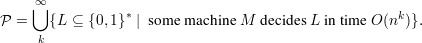
We take computability in polynomial time as our notion of “feasible computation”. Thus, consists of
those languages for which membership can be feasibly tested.

The complexity class is the set of languages for which membership can be proved in a feasible amount
of time. We say that a language L is in iff there is a relation RL(x,y) and polynomials p(n) and q(n)
with the following properties:
{0,1}*∣∃y {0,1}*(|y|≤ q(|x|) ∧ RL(x,y))}.We say that y is a witness to x’s membership in L iff |y|≤ q(|x|) and RL(x,y) is true. Thus, x L iff there
exists a witness to its membership in L. We can think of y as a “proof” that x L and the machine
computing RL as a verifier for the correctness of such proofs.
In summary, consists of those languages for which membership can be tested in a feasible amount of
time, and consists of those language for which polynomial length proofs of membership can be
verified in a feasible amount of time.
To test your understanding make sure you can prove the following:
Theorem 5 (easy) ⊆.