13 A Careful Proof of ⊆∕poly

We supply the missing piece to the proof of Theorem 4 in section 11 that ⊆∕poly. Namely, if L , there exists a ppTM M′ recognizing L with error probability less than 2^-n for all inputs x of length n.

Proof: By definition of , there exists a ppTM M that recognizes L with error probability at most 1∕3 for each input x. We can assume without loss of generality that M always outputs either 0 or 1.

Let r be an odd positive integer to be determined later. The ppTM M′ on input x of length n runs M(x) a total of r times and gives as its output the majority value among the multiset of r outputs from M. We use the Chernoff bound (see lecture 1)

(1)

plus additional probabilistic reasoning to bound the error probability of M′.

Define a random variable:

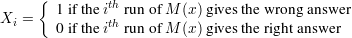
The number of wrong answers in computing M′(x) is ∑ X_i, so M′(x) gives the wrong answer iff ∑ X_i > r∕2.

We now calculate an upper bound on the error probability for M′(x). Let p be the probability that M(x) gives the wrong answer.¹ By assumption, p ≤ 1∕3.

Taking ε = 1∕6 and using the fact that p(1 - p) < 2∕9, equation 1 yields

(6)

It is easily verified that

(7)

for all r > 16(1 + n)∕log ₂e.

We now fix r to be the least odd positive integer satisfying equation 7. Combining equations 2–7 gives the desired error bound:

(8)

Moreover, M′ runs in polynomial time since M does and r = O(n). This establishes the lemma. __

14 One-Way Functions

One-way functions are at the heart of cryptography. Intuitively, a function f : {0,1}^*→{0,1}^* is one-way if it is “easy” to compute and “hard” to “invert”. We next give precise technical definitions of these concepts.

14.1 Strongly one-way functions

Definition: The function f is strongly one-way if it satisfies the following conditions:

1. f is computable in polynomial time.
2. For all probabilistic polynomial-time algorithms A′, all positive polynomials p(⋅), and all sufficiently large n,

   (9)

Intuitively, condition 2 says that any algorithm A′ that attempts to invert f has success probability less than one over any positive polynomial for all but finitely many n. Moreover, this fact remains true even when A′ is given additional information about the inverse that it is trying to find.

The notation of equation 9 is very compressed and deserves some explanation. First of all, U_n is the uniformly distributed random variable on binary strings of length n. Each occurrence of U_n refers to the same length-n random string x, so each occurrence of f(U_n) refers to same random string y = f(x). While x is uniformly distributed among all strings of length n, y is not so distributed. We are not assuming at this point that f is length preserving or that all strings x of length n map onto y’s of the same length. Moreover, f is not assumed to be one-to-one, so Pr[f(U_n) = y] = m2^-n, where m is the number of length n strings that f maps to y.

Because we don’t assume f is one-to-one, the notation f^-1(y) refers to a set rather than to a particular string. By definition,

This set is called the pre-image of y. Note that if y = f(x), then x f^-1(y), but there may be other strings in the pre-iamge as well.

With this background, we see that the event within the square brackets of equation 9 is the event that A′ succeeds in outputting some member of the pre-image f^-1(y) for a randomly chosen string y as described above. Condition 2 then says that this probability that this event occurs is negligible (according to the definition of “negligible” in section 10). Note that A′ is not required to output the string x that was used to generate y; any string in the pre-image will do.

Note also that A′ is told the length of x as its second input. Even with this additional help, A′ has only negligible success probability. This is done to prevent functions from being considered one-way only because their inverses are too long to output in a polynomial amount of time, e.g., the function g(x) = ℓ, where ℓ is the length of x written as a binary number. For example, g(111010111) = 1001 since |111010111| = 9, and (1001)₂ = 9.

14.2 Two obvious algorithms

Here are two obvious algorithms for inverting a function f.

1. Random guess. A₁(y,1ⁿ) outputs U_n, a uniformly distributed random string of length n. This is correct with probability at least 2^-n since there is a string x of length n such that f(x) = y, and A₁ has one chance in 2ⁿ of finding it. It will be correct with probability strictly greater than 2^-n if there is more than one string of length n that f maps to y. In particularly, for the function f that maps every string to a constant c, A₁ will be correct with probability 1.
2. Constant output. A₂(y,1ⁿ) outputs the string x₀ = 0ⁿ for every input of length n. This also is correct with probability at least 2^-n but for a different reason than A₁. Let y₀ = f(x₀). Then A₂(y) is correct when y = y₀. Since x is chosen uniformly at random from length-n strings, the probability that y = y₀ is at least 2^-n. As before, the probability will be greater if there is more than one string of length n that f maps to y₀. In particular, for the constant function f that maps every string to y₀, A₂ will be correct with probability 1.

Of course, to be strongly one-way, every p.p.t. algorithm A′ to invert f must have only a negligible probability of success, not just these two algorithms. But these examples provide a lower bound on what we can expect from a one-way function. In particular, no function can have an inversion success probability smaller than 2^-n.

14.3 Weakly one-way functions

We now define a much weaker version of a one-way function. While uninteresting for cryptographic purposes, we will show that the existence of weakly one-way functions implies the existence of strongly one-way functions.

Definition: The function f is weakly one-way if it satisfies the following conditions:

1. f is computable in polynomial time.
2. There exists a positive polynomial p(⋅) such that for all probabilistic polynomial-time algorithms A′ and all sufficiently large n,

   (10)

Note the subtle change in the order of quantifiers and in equation 10. This says that any algorithm A′ that attempts to invert f will take a noticeable amount of the time on inputs of length n for all sufficiently large n.

A function μ(n) is noticeable if μ(n) > 1∕p(n) for some fixed positive polynomial p(⋅) and all sufficiently large n. A function cannot be both noticeable and negligible, but it is possible for a function to be neither. For example, the function μ(n) = n mod 2 that equals 1 on all odd numbers and 0 on all even numbers is neither negligible nor noticeable. It is not negligible because it fails to be smaller than 1∕p(n) for infinitely many n, where p(n) = 2. It is not noticeable because it fails to be larger than 1∕q(n) > 0 for infinitely many n and all positive polynomials q(n).