
YALE UNIVERSITY
DEPARTMENT OF COMPUTER SCIENCE
| CPSC 461b: Foundations of Cryptography | Notes 14 (rev. 1) | |
| Professor M. J. Fischer | February 26, 2009 | |
Lecture Notes 14
Let ℓ(n) = n. We show how to construct an efficiently computable ℓ-bit pseudorandom function ensemble, starting from a pseudorandom generator G with expansion factor 2n.
Let s be an n-bit string, so G(s) is a 2n-bit string. Define G0(s) (resp. G1(s)) to be the first (resp. last) n bits of G(s). Define a function fs : {0,1}n →{0,1}n as follows: For every σ = σ1σ2…σn of length n, let
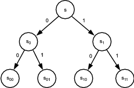
The construction of fs can be represented by a tree, the first three levels of which are shown in Figure 35.1. Each node on level k is labeled by an n-bit string sτ, where τ is a string of length k. The left son of node sτ is labeled by sτ0 = G0(sτ), and the right son is labeled by sτ1 = G1(sτ). The leaf label sσ is the value of the function fs(σ).
Let Fn be the random variable that selects s uniformly from {0,1}n, places it at the root of the
tree, and then generates the labels of the remaining nodes as described above to obtain the
resulting function fs. Let F = {Fn}n ℕ be the function ensemble that corresponds to this random
process.
ℕ be the function ensemble that corresponds to this random
process.
Theorem 1 If G is a pseudorandom generator, then F is an efficiently computable ensemble of pseudorandom functions.
The kth hybrid Hnk is a random variable ranging over functions that assign labels uniformly at the kth level of the tree. In more detail, Hnk selects sτ uniformly from {0,1}n for each τ of length k and places those 2k values in the corresponding nodes of level k of the tree. It then generates the labels of the nodes below level k using the functions G0 and G1 as described above. The leaves of the tree define the resulting function, which in turn is uniquely determined by the level-k node labels sτ1,…sτ 2k. We denote this function by

(Note that the nodes at levels less than k do not get labeled by this process, but only the leaves are relevant to the defined function.)
By this construction, we have Hn0 = Fn, the original pseudorandom function construction, and Hnn = Hn, the uniform distribution over functions {0,1}n →{0,1}n.
Now, assume that F is not pseudorandom. Then there exists a probabilistic polynomial-time oracle machine M and a positive polynomial p(⋅) such that for infinitely many n,
![Fn n Hn n 1
Δ (n ) = |Pr[M (1 ) = 1]- P r[M (1 ) = 1]| > p(n-).](ln143x.png)
Let t(⋅) be a polynomial bound on the running time of M(1n). It follows that M(1n) makes at most t(n) queries of its oracle.
We construct a probabilistic polynomial-time distinguisher D that distinguishes t(n) samples from
{G(Un)}nℕ from t(n) samples from {U2n}nℕ with non-negligible advantage.
Algorithm D on input α1,…,αt(n)  {0,1}2n: {0,1}2n:
|
| 1. | Select k uniformly from {0,1,…,n - 1}. |
| 2. | Run M(1n) and output its result. Answer each of its oracle queries as described below. |
The idea is that the oracle queries should be answered according to a tree that is dynamically constructed during the execution of D. Initially, all nodes are unlabeled. For each query qi = σ1…σn, the nodes at levels > k that lie on the path qi receive labels, as well as the brother of the level-(k + 1) node that lies on that path. Once a node is labeled, it retains that label throughout the duration of the run.
The labeling in turn works as follows. If the level-(k + 1) node (σ1…σkσk+1) has not yet been labeled, it and its brother are labeled using input string αi as follows:
where for any string y of length 2n, P0(y) is the left half of y and P1(y) is the right half of y.1 The nodes below (σ1…σk+1) are labeled as usual using G, i.e.,

for each j = k+2,…,n.2
Observe that when the inputs to D are t(n) samples from U2n, then P0(αi) and P1(αi) are both uniformly distributed. This means that whenever a node on level-(k + 1) receives a label, the label is uniformly distributed. Hence, D behaves as M would given oracle Hnk+1.
When the inputs to D are t(n) samples from G(Un), then the nodes on level-(k + 1) are labeled according to G0(s) and G1(s) for randomly chosen s. That is, if αi = G(Un), then there is some s such that αi = G(s). The construction sets sτ0 = Po(αi) = G0(s) and sτ1 = Po(αi) = G1(s), so D behaves as M would given oracle Hnk. Note that D does not actually label node τ with s, nor is it able to compute s from αi, but the nodes below τ are labeled just as if node τ were labeled by s.
The following claims relate the success probability of D to the probability that M outputs 1. In both claims, K is the random value chosen in step 1 of Algorithm D.
By the hybrid argument, since Δ(n) >  , it follows that
![Hkn n Hkn+1 n Δ-(n) ---1---
|Pr[M ( ) = 1]- P r[M (1 ) = 1]| ≥ n > n ⋅p(n)](ln149x.png)
for some k. Since also Pr[K = k] =  , we have from claims 1 and 2 that
![(1) (t(n)) (1) (t(n)) 1
|Pr[D (G(Un ),...,G (Un )) = 1]- P r[D (U2n ),...,U 2n )) = 1]| > n2 ⋅p(n).](ln1411x.png)
Thus, D distinguishes with inverse polynomial advantage and polynomially many samples between
G(Un) and U2n. Since {G(Un)}nℕ and {U2n}nℕ are both efficiently constructible ensembles, it follows
from Theorem 3 in section 28.2 of lecture 11 (Theorem 3.2.6 of the textbook) that G(Un) and U2n are
distinguishable in polynomial time by a single sample with polynomial advantage. Hence, G is not
pseudorandom, a contradiction.
We conclude that F is an efficiently computable ensemble of pseudorandom functions, as desired. __
Here’s a simple example from the textbook of an application of a pseudorandom function ensemble F . Suppose a a secret society wants a way to identify its members. Imagine each club member is given the secret seed s that defines a function fs = Fn. Members are instructed never to divulge s. Rather, to authenticate someone claiming to be a member, ask them to tell you the value of the secret function fs on a random challenge string x. You also compute fs(x) and accept the person as a member if the two values agree. Note that you are giving away very little information on each such authentication. It can be shown that an adversary succeeds with negligible probability, even after a polynomial number of attempts. If not, the adversary can be used to distinguish F from H. (See section 3.6.3 of the textbook for further details.)
![(1) (t(n)) k
P r[D(G (Un ),...,G (U n )) = 1 | K = k] = Pr[M Hn(n) = 1].](ln146x.png)
![P r[D(U (12n)),...,U (2t(nn)))) = 1 | K = k] = Pr[M Hkn+1(1n) = 1].](ln147x.png)