114 Bit-prediction

One important property of the uniform distribution U on bit-strings b₁,…,b_ℓ is that the individual bits are statistically independent from each other. This means that the probability that a particular bit b_i = 1 is unaffected by the values of the other bits in the sequence. Thus, any algorithm that attempts to predict b_i, even knowing other bits of the sequence, will be correct only 1/2 of the time. We now translate this property of unpredictability to pseudorandom sequences.

114.1 Next-bit prediction

One property we would like a pseudorandom sequence to have is that it be difficult to predict the next bit given the bits that came before.

We say that an algorithm A is an ε-next-bit predictor for bit i of a PRSG G if

where (b₁,…,b_i) = G_i(S). To explain this notation, S is a uniformly distributed random variable ranging over the possible seeds for G. G(S) is a random variable (i.e., probability distribution) over the output strings of G, and G_i(S) is the corresponding probability distribution on the length-i prefixes of G(S).

Next-bit prediction is closely related to indistinguishability, introduced in section 110. We will show later that if if G(S) has a next-bit predictor for some bit i, then G(S) is distinguishable from the uniform distribution U on the same length strings, and conversely, if G(S) is distinguishable from U, then there is a next-bit predictor for some bit i of G(S). The precise definitions under which this theorem is true are subtle, for one must quantify both the amount of time the judge and next-bit predictor algorithms are permitted to run as well as how much better than chance the judgments or predictions must be in order to be considered a successful judge or next-bit predictor. We defer the mathematics for now and focus instead on the intuitive concepts that underlie this theorem.

114.2 Building a judge from a next-bit predictor

Suppose a PRSG G has an ε-next-bit predictor A for some bit i. Here’s how to build a judge J that distinguishes G(S) from U. The judge J, given a sample string drawn from either G(S) or from U, runs algorithm A to guess bit b_i from bits b₁,…,b_i-1. If the guess agrees with the real b_i, then J outputs 1 (meaning that he guesses the sequence came from G(S)). Otherwise, J outputs 0. For sequences drawn from G(S), J will output 1 with the same probability that A successfully predicts bit b_i, which is at least 1∕2 + ε. For sequences drawn from U, the judge will output 1 with probability exactly 1/2. Hence, the judge distinguishes G(S) from U with advantage ε.

It follows that no cryptographically strong PRSG can have an ε-next-bit predictor. In other words, no algorithm that attempts to predict the next bit can have more than a “small” advantage ε over chance.

114.3 Previous-bit prediction

Previous-bit prediction, while perhaps less natural, is analogous to next-bit prediction. An ε-previous-bit predictor for bit i is an algorithm that, given bits b_i+1,…,b_ℓ, correctly predicts b_i with probability at least 1∕2 + ε.

As with next-bit predictors, it is the case that if G(S) has a previous-bit predictor for some bit b_j, then some judge distinguishes G(S) from U. Again, I am being vague with the exact conditions under which this is true. The somewhat surprising fact follows that G(S) has an ε-next-bit predictor for some bit i if and only if it has an ε′-previous-bit predictor for some bit j (where ε and ε′ are related but not necessarily equal).

To give some intuition into why such a fact might be true, we look at the special case of ℓ = 2, that is, of 2-bit sequences. The probability distribution G(S) can be described by four probabilities

Written in tabular form, we have

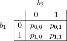
We describe an algorithm A(v) for predicting b₁ given b₂ = v. A(v) predicts b₁ = 0 if p_0,v > p_1,v, and it predicts b₁ = 1 if p_0,v ≤ p_1,v. In other words, the algorithm chooses the value for b₁ that is most likely given that b₂ = v. Let a(v) be the value predicted by A(v).

Proof: Assume A is an ε-previous-bit predictor for b₁. Then A correctly predicts b₁ given b₂ with probability at least 1∕2 + ε. We show that A is an ε-next-bit predictor for either b₁ or b₂.

We have two cases:

Case 1: a(0) = a(1). Then algorithm A does not depend on v, so A itself is also an ε-next-bit predictor for b₁.

Case 2: a(0)a(1). The probability that A(v) correctly predicts b₁ when b₂ = v is given by the conditional probability

The overall probability that A(b₂) is correct for b₁ is the weighted average of the conditional probabilities for v = 0 and v = 1, weighted by the probability that b₂ = v. Thus,

Now, since a(0)a(1), the function a is one-to-one and onto. A simple case analysis shows that either a(v) = v for v {0,1}, or a(v) = ¬v for v {0,1}. That is, a is either the identity or the complement function. In either case, a is its own inverse. Hence, we may also use algorithm A(u) as a predictor for b₂ given b₁ = u. By a similar analysis to that used above, we get

since either a is the identity function or the complement function. Hence, A(b₁) is correct for b₂ with the same probability that A(b₂) is correct for b₁. Therefore, A is an ε-next-bit predictor for b₂.

In both cases, we conclude that A is an ε-next-bit predictor for either b₁ or b₂. __

115 Foundations of Cryptography

[This section is based on the second textbook, John Talbot and Dominic Welsh, Complexity and Cryptograpy: An Introduction, §6.1–6.3.]

We have been rather vague throughout the course about what it means for a problem to be “hard” to solve. A public key system such as RSA can always be broken given enough time. Eve could simply factor n and find the decryption key, or she could try all possible messages m to see which one encrypts to the known ciphertext c given the public encryption key. So we can’t hope to always prevent Eve from decrypting our messages. The best we can hope for is that she rarely succeeds. We can state this as follows:

We have to say what “negligible” means. A function r : ℕ → ℕ is negligible if for all polynomial functions p : ℕ → ℕ, there exists k₀ such that for all k ≥ k₀,

(We assume p(k) ≥ 1 for all integers k ≥ 0.)

This definition says that r(k) → 0 as k →∞. But it says more. It also says that r(k) goes to 0 “faster” than one over any polynomial. For all large enough k, r(k) is smaller than 1∕k¹⁰, for example. It’s tempting to equate negligible with inverse exponential. While 1∕2^k is indeed a negligible function, there are larger functions that are also negligible by our definitions, for example, 1∕2 and 1∕k^{log k}.

Definition: A function f is strong one-way if

1. f is polynomial time computable.
2. Any probabilistic polynomial time algorithm for inverting f(x) when given a random instance y = f(x) has negligible chance of finding a preimage of y.

By “random instance”, this means a y of the form y = f(x) for a uniformly distributed random x.

Even this definition hides some technical difficulties that are done carefully in the text book. In particular, the difficulty of inverting f should remain hard even when the inverter is told the length of x.

The following function related to the discrete log problem is often assumed to be strong one:

It is easy to compute, but to invert it requires solving the discrete log problem.

Although functions like dexp and factoring are believed to be strong one-way functions, no function has been proved to be strong one-way. The following theorem explains why it is so hard to prove that functions are strong one-way – doing so would also settle the famous P = NP? problem by showing that PNP .

Proof: Assume f is strong one-way. Define the language

L_f is easily seen to be in NP . To test if a given (x,y,1^k) triple is in L_f, simply guess a string u of length k, compute f(xu), and check that f(xu) = y.

If P = NP , then there is a polynomial time algorithm A for testing membership in L_f. A can be used to determine the bits of a preimage of y one by one. At stage i, assume that the first i-1 bits x_i-1 of a preimage have already been determined. To determine bit i, test if (x_i-10,y,1^k-i) L_f. If so, then x_i = 0x_i-1 are the first i bits of some preimage. If not, then (x_i-11,y,1⁽k - i)) must be in L_f since x_i01 is known to be the prefix of a preimage. Hence, one can take x_i = x_i-11 in this case. After stage k, the number x_k is a preimage of y, as desired. The entire procedure requires only k evaluations of A, so it is also a polynomial time algorithm for inverting f, contradicting the assumption that f is one-way.

We conclude that PNP if one-way functions exist. __