68 Legendre Symbol

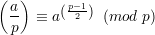
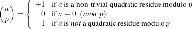
Let p be an odd prime, a an integer. The Legendre symbol is a number in {-1,0,+1}, defined as follows:

By the Euler Criterion (see Claim 3), we have

Theorem 1 Let p be an odd prime. Then

Note that this theorem holds even when p∣a.

The Legendre symbol satisfies the following multiplicative property: Fact Let p be an odd prime. Then

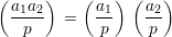
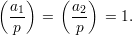
Not surprisingly, if a₁ and a₂ are both non-trivial quadratic residues, then so is a₁a₂. This shows that the fact is true for the case that

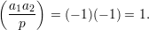
More surprising is the case when neither a₁ nor a₂ are quadratic residues, so

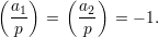
In this case, the above fact says that the product a₁a₂ is a quadratic residue since

Here’s a way to see this. Let g be a primitive root of p. Write a₁ ≡ g^k₁ (mod p) and a₂ ≡ g^k₂ (mod p). Since a₁ and a₂ are not quadratic residues, it must be the case that k₁ and k₂ are both odd; otherwise g^k₁∕2 would be a square root of a₁, or g^k₂∕2 would be a square root of a₂. But then k₁ + k₂ is even since the sum of any two odd numbers is always even. Hence, g^{(k₁+k₂)∕2} is a square root of a₁a₂ ≡ g^k₁+k₂ (mod p), so a₁a₂ is a quadratic residue.

69 Jacobi Symbol

The Jacobi symbol extends the Legendre symbol to the case where the “denominator” is an arbitrary odd positive number n.

Let n be an odd positive integer with prime factorization ∏ _i=1^kp_i^e_i. We define the Jacobi symbol by

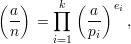(1)

where the symbol on the left is the Jacobi symbol, and the symbol on the right is the Legendre symbol. (By convention, this product is 1 when k = 0, so = 1.) Clearly, when n = p is an odd prime, the Jacobi symbol and Legendre symbols agree, so the Jacobi symbol is a true extension of our earlier notion.

What does the Jacobi symbol mean when n is not prime? If = -1 then a is definitely not a quadratic residue modulo n, but if = 1, a might or might not be a quadratic residue.

Consider the important case of n = pq for p, q distinct odd primes. Then

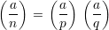(2)

so there are two cases that result in = 1: either = = +1 or = = -1.

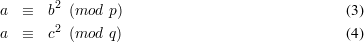
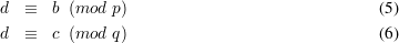
In the first case, a is a quadratic residue modulo both p and q, so a is a quadratic residue modulo n. Let b and c be square roots of a modulo p and q, respectively, so

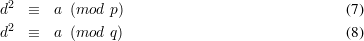
In the second case, a is not a quadratic residue modulo either p or q, so it is not a quadratic residue modulo n, either. Such numbers a are sometimes called “pseudo-squares” since they have Jacobi symbol 1 but are not quadratic residues.

70 Identities Involving the Jacobi Symbol

The Jacobi symbol is easily computed using Equation 1 of section 69 and Theorem 1 of section 68 if the factorization of n is known. Similarly, gcd(u,v) is easily computed without resort to the Euclidean algorithm given the factorizations of u and v. The remarkable fact about the Euclidean algorithm is that it lets us compute gcd(u,v) efficiently even without knowing the factors of u and v. A similar algorithm allows the Jacobi symbol to be computed efficiently without knowing the factorization of a or n.

The algorithm is based on identities satisfied by the Jacobi symbol:

1. = 1; = 0 for n≠1;
2. = 1 if n ≡±1 (mod 8); = -1 if n ≡±3 (mod 8);
3. = if a₁ ≡ a₂ (mod n);
4. = ;
5. = - if a ≡ n ≡ 3 (mod 4).
6. = if a ≡ 1 (mod 4) or (a ≡ 3 (mod 4) and n ≡ 1 (mod 4));

There are many ways to turn these identities into an algorithm. Below is a straightforward recursive approach. Slightly more efficient iterative implementations are also possible.

71 Solovay-Strassen Test of Compositeness

Recall that a test of compositeness for n is a set of predicates {τ_a(n)}_aZ*n such that if τ(n) succeeds (is true), then n is composite. The Solovay-Strassen Test is the set of predicates {ν_a(n)}_aZ*n, where

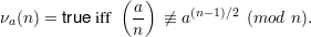
If n is prime, the test always fails by Theorem 1 of section 68. Equivalently, if some ν_a(n) succeeds, then n must be composite. Hence, the test is a valid- test of compositeness.

Let b = a^(n-1)∕2, so b² ≡ a^n-1. There are two possible reasons why the test might succeed. One possibility is that a^n-1 ⁄≡ 1 (mod n) in which case b ⁄≡±1 (mod n). This is just the Fermat test ζ_a(n) from section 52 of lecture notes 12. A second possibility is that a^n-1 ≡ 1 (mod n) but nevertheless, b ⁄≡ (mod n). In this case, b is a square root of 1 (mod n), but it might have the opposite sign from , or it might not even be ±1 since 1 has additional square roots when n is composite. Strassen and Solovay show the probability that ν_a(n) succeeds for a randomly-chosen a Z*_n is at least 1∕2 when n is composite.¹

72 Miller-Rabin Test of Compositeness

The Miller-Rabin Test is more complicated to describe than the Solovay-Strassen Test, but the probability of error (that is, the probability that it fails when n is composite) seems to be lower than for Solovay-Strassen, so that the same degree of confidence can be achieved using fewer iterations of the test. This makes it faster when incorporated into a primality-testing algorithm. It is also closely related to the algorithm presented in section 56.3 (lecture notes 13) for factoring an RSA modulus given the encryption and decryption keys and to Shanks Algorithm 66.1 (lecture notes 15) for computing square roots modulo an odd prime.

72.1 The test

The test μ_a(n) is based on computing a sequence b₀,b₁,…,b_s of integers in Z*_n. If n is prime, this sequence ends in 1, and the last non-1 element, if any, is n- 1 (≡-1 (mod n)). If the observed sequence is not of this form, then n is composite, and the Miller-Rabin Test succeeds. Otherwise, the test fails.

The sequence is computed as follows:

1. Write n - 1 = 2^st, where t is an odd positive integer. Computationally, s is the number of 0’s at the right (low-order) end of the binary expansion of n, and t is the number that results from n when the s low-order 0’s are removed.
2. Let b₀ = a^t mod n.
3. For i = 1,2,…,s, let b_i = (b_i-1)² mod n.

An easy inductive proof shows that b_i = a^2it mod n for all i, 0 ≤ i ≤ s. In particular, b_s ≡ a^2st = a^n-1 (mod n).

72.2 Validity

To see that the test is valid, we must show that μ_a(p) fails for all a Z*_p when n is a prime p. By Euler’s theorem² , a^p-1 ≡ 1 (mod p), so we see that b_s = 1. Since 1 has only two square roots modulo p, 1 and -1, and b_i-1 is a square root of b_i modulo p, the last non-1 element in the sequence (if any) must be -1 mod p. This is exactly the condition for which the Miller-Rabin test fails. Hence, it fails whenever n is prime, so if it succeeds, n is indeed composite.

72.3 Accuracy

How likely is it to succeed when n is composite? It succeeds whenever a^n-1 ⁄≡ 1 (mod n), so it succeeds whenever the Fermat test ζ_a(n) would succeed. (See section 52 of lecture notes 12.) But even when a^n-1 ≡ 1 (mod n) and the Fermat test fails, the Miller-Rabin test will succeed if the last non-1 element in the sequence of b’s is one of the two square roots of 1 that differ from ±1. It can be proved that μ_a(n) succeeds for at least 3∕4 of the possible values of a. Empirically, the test almost always succeeds when n is composite, and one has to work to find a such that μ_a(n) fails.

72.4 Example

For example, take n = 561 = 3 ⋅ 11 ⋅ 17. This number is interesting because it is the first Carmichael number. A Carmichael number is an odd composite number n that satisfies a^n-1 ≡ 1 (mod n) for all a Z*_n. (See http://mathworld.wolfram.com/CarmichaelNumber.html.) These are the numbers that I have been calling “pseudoprimes”. Let’s go through the steps of computing μ₃₇(561).

We begin by finding t and s. 561 in binary is 1000110001 (a palindrome!). Then n-1 = 560 = (1000110000)₂, so s = 4 and t = (100011)₂ = 35. We compute b₀ = a^t = 37³⁵ mod 561 = 265 with the help of the computer. We now compute the sequence of b’s, also with the help of the computer. The results are shown in the table below:

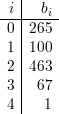
This sequence ends in 1, but the last non-1 element b₃ ⁄≡-1 (mod 561), so the test μ₃₇(561) succeeds. In fact, the test succeeds for every a Z*₅₆₁ except for a = 1,103,256,460,511. For each of those values, b₀ = a^t ≡ 1 (mod 561).

72.5 Optimization

In practice, one only wants to compute as many of the b’s as necessary to determine whether or not the test succeeds. In particular, one can stop after computing b_i if b_i ≡±1 (mod n). If b_i ≡-1 (mod n) and i < s, the test fails. If b_i ≡ 1 (mod n) and i ≥ 1, the test succeeds. This is because we know in this case that b_i-1 ⁄≡-1 (mod n), for if it were, the algorithm would have stopped after computing b_i-1.