April 6 - More Learning - Ensemble and Adaboost
Mostly chapter 18 and 20 from AIMA
from learning import *
from notebook import *
ENSEMBLE LEARNER
Overview
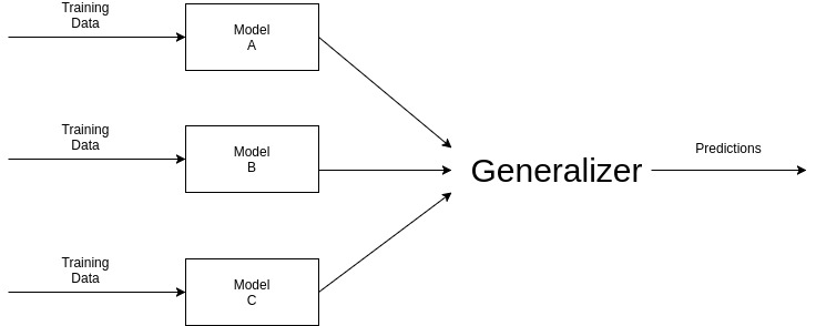
Ensemble Learning improves the performance of our model by combining several learners. It improves the stability and predictive power of the model. Ensemble methods are meta-algorithms that combine several machine learning techniques into one predictive model in order to decrease variance, bias, or improve predictions.
Some commonly used Ensemble Learning techniques are :
Bagging : Bagging tries to implement similar learners on small sample populations and then takes a mean of all the predictions. It helps us to reduce variance error.
Boosting : Boosting is an iterative technique which adjust the weight of an observation based on the last classification. If an observation was classified incorrectly, it tries to increase the weight of this observation and vice versa. It helps us to reduce bias error.
Stacking : This is a very interesting way of combining models. Here we use a learner to combine output from different learners. It can either decrease bias or variance error depending on the learners we use.
Implementation
Below mentioned is the implementation of Ensemble Learner.
psource(EnsembleLearner)
This algorithm takes input as a list of learning algorithms, have them vote and then finally returns the predicted result.
LEARNER EVALUATION
In this section we will evaluate and compare algorithm performance. The dataset we will use will again be the iris one.
iris = DataSet(name="iris")
Naive Bayes
First up we have the Naive Bayes algorithm. First we will test how well the Discrete Naive Bayes works, and then how the Continuous fares.
nBD = NaiveBayesLearner(iris, continuous=False)
print("Error ratio for Discrete:", err_ratio(nBD, iris))

nBC = NaiveBayesLearner(iris, continuous=True)
print("Error ratio for Continuous:", err_ratio(nBC, iris))
The error for the Naive Bayes algorithm is very, very low; close to 0. There is also very little difference between the discrete and continuous version of the algorithm.
k-Nearest Neighbors
Now we will take a look at kNN, for different values of k. Note that k should have odd values, to break any ties between two classes.
kNN_1 = NearestNeighborLearner(iris, k=1)
kNN_3 = NearestNeighborLearner(iris, k=3)
kNN_5 = NearestNeighborLearner(iris, k=5)
kNN_7 = NearestNeighborLearner(iris, k=7)

print("Error ratio for k=1:", err_ratio(kNN_1, iris))
print("Error ratio for k=3:", err_ratio(kNN_3, iris))
print("Error ratio for k=5:", err_ratio(kNN_5, iris))
print("Error ratio for k=7:", err_ratio(kNN_7, iris))
Notice how the error became larger and larger as k increased. This is generally the case with datasets where classes are spaced out, as is the case with the iris dataset. If items from different classes were closer together, classification would be more difficult. Usually a value of 1, 3 or 5 for k suffices.
Also note that since the training set is also the testing set, for k equal to 1 we get a perfect score, since the item we want to classify each time is already in the dataset and its closest neighbor is itself.
Perceptron
For the Perceptron, we first need to convert class names to integers. Let's see how it performs in the dataset.
iris2 = DataSet(name="iris")
iris2.classes_to_numbers()

perceptron = PerceptronLearner(iris2)
print("Error ratio for Perceptron:", err_ratio(perceptron, iris2))
The Perceptron didn't fare very well mainly because the dataset is not linearly separated. On simpler datasets the algorithm performs much better, but unfortunately such datasets are rare in real life scenarios.
AdaBoost
Overview
AdaBoost is an algorithm which uses ensemble learning. In ensemble learning the hypotheses in the collection, or ensemble, vote for what the output should be and the output with the majority votes is selected as the final answer.
AdaBoost algorithm, as mentioned in the book, works with a weighted training set and weak learners (classifiers that have about 50%+epsilon accuracy i.e slightly better than random guessing). It manipulates the weights attached to the examples that are showed to it. Importance is given to the examples with higher weights.
One way to think about this is that you have more to learn from your mistakes than from your success. If you predict X and are correct, you have nothing to learn.If you predict X and are wrong, you made a mistake. You need to update your model. You have something to learn. In the cognitive science world, this is known as failure-driven learning. It is a powerful notion. Think about it. How do you know that you have something to learn? You make a mistake. You expected one outcome and something else happened. Actually, you do not need to make a mistake. Suppose you try something and expect to fail. If you actually succeed, you still have something to learn because you had an **expectation failure**.
All the examples start with equal weights and a hypothesis is generated using these examples. Examples which are incorrectly classified, their weights are increased so that they can be classified correctly by the next hypothesis. The examples that are correctly classified, their weights are reduced. This process is repeated K times (here K is an input to the algorithm) and hence, K hypotheses are generated.
These K hypotheses are also assigned weights according to their performance on the weighted training set. The final ensemble hypothesis is the weighted-majority combination of these K hypotheses.
The speciality of AdaBoost is that by using weak learners and a sufficiently large K, a highly accurate classifier can be learned irrespective of the complexity of the function being learned or the dullness of the hypothesis space.
Implementation
As seen in the previous section, the PerceptronLearner does not perform that well on the iris dataset. We'll use perceptron as the learner for the AdaBoost algorithm and try to increase the accuracy.
Let's first see what AdaBoost is exactly:
psource(AdaBoost)
AdaBoost takes as inputs: L and K where L is the learner and K is the number of hypotheses to be generated. The learner L takes in as inputs: a dataset and the weights associated with the examples in the dataset. But the PerceptronLearner doesnot handle weights and only takes a dataset as its input.
To remedy that we will give as input to the PerceptronLearner a modified dataset in which the examples will be repeated according to the weights associated to them. Intuitively, what this will do is force the learner to repeatedly learn the same example again and again until it can classify it correctly.
To convert PerceptronLearner so that it can take weights as input too, we will have to pass it through the WeightedLearner function.
psource(WeightedLearner)
The WeightedLearner function will then call the PerceptronLearner, during each iteration, with the modified dataset which contains the examples according to the weights associated with them.
Example
We will pass the PerceptronLearner through WeightedLearner function. Then we will create an AdaboostLearner classifier with number of hypotheses or K equal to 5.
WeightedPerceptron = WeightedLearner(PerceptronLearner)
AdaboostLearner = AdaBoost(WeightedPerceptron, 5)
iris2 = DataSet(name="iris")
iris2.classes_to_numbers()

adaboost = AdaboostLearner(iris2)

adaboost([5, 3, 1, 0.1])
That is the correct answer. Let's check the error rate of adaboost with perceptron.
print("Error ratio for adaboost: ", err_ratio(adaboost, iris2))
It reduced the error rate considerably. Unlike the PerceptronLearner, AdaBoost was able to learn the complexity in the iris dataset.
psource(err_ratio)