YALE UNIVERSITY
DEPARTMENT OF COMPUTER SCIENCE
| CPSC 461b: Foundations of Cryptography | Notes 10 (rev. 1) | |
| Professor M. J. Fischer | February 12, 2009 | |
Lecture Notes 10
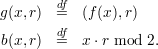
We now complete the proof of Lemma 3 of section 21. Recall again that f is a strongly one-way and length preserving function and that
Assuming that b is not a hard core for g, there is a p.p.t. algorithm G and a polynomial p(n) such that G predicts b with advantage
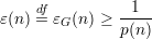 | (1) |
for all n in an infinite set N. In section 22.2 of lecture 9, we constructed an algorithm A for inverting f.
We now show that A has success probability at least  at inverting f on length-n inputs, for all
n
at inverting f on length-n inputs, for all
n  N. This contradicts the assumption that f is strongly one-way and completes the proof of
Lemma 3.
N. This contradicts the assumption that f is strongly one-way and completes the proof of
Lemma 3.
Assume for the rest of this discussion that n N. Let
![s(x) = Pr[G (f (x ),Rn ) = b(x,Rn )].](ln103x.png)
Here Rn is a uniformly distributed random variable over length-n strings, distinct from the identically distributed random variables Un and Xn, which we also mention from time to time. Thus, s(x) is the fine-grained success probability of G for each particular length-n string x. We know that the average of s(x) taken over all length-n strings x is the overall success probability of G, so
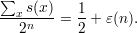 | (2) |
Define
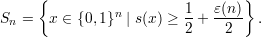 | (3) |
Three different proofs of this claim are given in handout 3: One is algebraic, one is geometric, and one
is based on Markov’s inequality. We do not repeat them here but refer the reader to the handout. We only
mention that all three are based on the idea that in order for the average value of s(x) to exceed  + ε(n),
there must be a certain number of x for which s(x) ≥
+ ε(n),
there must be a certain number of x for which s(x) ≥ +
+  . That number turns out to be
ε(n) ⋅ 2n.
. That number turns out to be
ε(n) ⋅ 2n.
Proof: Let x Sn and i {1,…,n}. Let ζJ be a random variable ranging over {0,1} such that
![J 1- ε(n) 1- --1--
P r[ζ = 1] = s(x) ≥ 2 + 2 ≥ 2 + 2p (n ).](ln1011x.png) | (4) |
A key observation is that the ζJ’s are pairwise independent. This follows from the fact that the rJ’s are
pairwise independent. To see this, let J≠K. Without loss of generality, we can choose k K - J. By
definition, rK and rJ are both sums of subsets of the independent random variables {s1,…,sℓ}. Since
k K -J, the term sk appears in the sum for rK but not for rJ. Therefore, sk is independent of rJ, which
implies that rK is independent of rJ.
Let m = 2ℓ - 1. Since ℓ = ⌈log 2(2n⋅p(n)2 + 1)⌉, we have that 2ℓ ≥ 2log 2(2n⋅p(n)2+1) = 2n⋅p(n)2 + 1, so m ≥ 2n ⋅ p(n)2. We also have
 | (5) |
We use Chebyshev’s inequality to bound Pr[∑
JζJ ≤ ⋅ m]. This is an upper bound on the
probability that the majority value zi that algorithm A computes for xi is wrong. Recall Chebyshev’s
inequality
⋅ m]. This is an upper bound on the
probability that the majority value zi that algorithm A computes for xi is wrong. Recall Chebyshev’s
inequality
![Var(X )
P r[|X - E(X )| ≥ δ] ≤---2---.
δ](ln1014x.png) | (6) |
Let X = ∑
JζJ and δ =  . All of the ζJ are identically distributed, so we drop the superscript in the
following.
. All of the ζJ are identically distributed, so we drop the superscript in the
following.
![1- --1--
E (ζ) = P r[ζ = 1] ≥ 2 + 2p(n)](ln1016x.png)
by equation 4. Thus,
 | (7) |
We also have
Since ζ is 0-1 valued, it follows that ζ2 = ζ. Hence,
The bound of 1∕4 simply reflects the fact that the maximum value of the function x(1 - x), which is reached for x = 1∕2. Since the variables ζJ are pairwise independent, they are also uncorrelated, so
 | (8) |
Plugging the expression for δ into inequality 6 and doing some calculations using inequalities 7 and 8, we get
![| |
[ 1 ] [| ( 1 1 ) | 1 ]
Pr X ≤ 2 ⋅m ≤ Pr ||X - 2 + 2p(n) ⋅m || ≥ 2p(n-) ⋅m
V-ar(X)-
≤ (-m--)2
2p(n)
m- (2p(n-))2- p-(n-)2
≤ 4 ⋅ m2 = m
p(n)2 1
≤ --------2 = --.
2n ⋅p(n) 2n](ln1021x.png)
To finish the proof of the lemma, we observe that A successfully inverts f(x) if all of the following are true:
Sn.
The first event is true with probability at least ε(n) ≥ by Claim 1. The second event is true with
probability
by Claim 1. The second event is true with
probability
by inequality 5. The third event is true with probability at least (1 - )n >
)n >  for all n ≥ 2. Multiplying
these together gives us a lower bound on the success probability of f, namely,
for all n ≥ 2. Multiplying
these together gives us a lower bound on the success probability of f, namely,
Thus, taking q(n) = 8n⋅p(n)3 + 4p(n), A has a success probability greater than  for all sufficiently
large n N, contradicting the assumption that f is strongly one-way. Thus, the assumption that b is
not hard-core for f and that G exists must be false. This completes the proof of Lemma 3 of
section 21.
for all sufficiently
large n N, contradicting the assumption that f is strongly one-way. Thus, the assumption that b is
not hard-core for f and that G exists must be false. This completes the proof of Lemma 3 of
section 21.
We extend the notion of a hard-core predicate of a function to a hard-core function.
Definition: Let h : {0,1}* → {0,1}* be a polynomial-time computable length-regular function.1 Let ℓ = |h(1n)|. h is a hard core of f if for all p.p.t. algorithms D′, all positive polynomials p(⋅), and all sufficiently large n,
![1
|P r[D ′(f (Xn ),h(Xn )) = 1]- P r[D ′(f(Xn),R ℓ(n)) = 1] <---,
p(n)](ln1028x.png)
where Xn and Rℓ(n) are independent random variables, uniformly distributed over {0,1}n and {0,1}ℓ(n), respectively.
Intuitively, h is a hard core for f if the value of h(x) is indistinguishable from a random string, even knowing the value of f(x). On the surface, this looks to be an even stronger condition than unpredictability. Obviously, if one could predict h(x) from f(x), then one could distinguish h(x) from random. Namely, if the given string equals the prediction, output 1, otherwise output 0. On the other hand, it’s not a priori obvious how being able to distinguish h(x) from random would be useful at prediction.
Theorem 1 Let f be strongly one-way. Let c > 0 and let ℓ(n) = min{n,⌈clog 2n⌉}. Let x be a string of length n and s a string of length 2n. Define
We omit the non-trivial proof of this theorem and remark only that hard core functions with logarithmic lengths are known for RSA and other cryptographic collections, assuming the corresponding collections are one-way. Details are in the textbook.
To begin our formal development of pseudorandom sequence generation, we define a probability ensemble, analogous to the previous definition of a collection of one-way functions.
Let I be a countable set. An ensemble indexed by I is a sequence of random variables X = {Xi}i I
indexed by I.
I
indexed by I.
Typical index sets are the natural numbers ℕ or binary strings {0,1}*. Typically, X = {Xn}nℕ has
Xn ranging over strings of length poly(n), and X = {Xw}w{0,1}* has Xw ranging over strings of length
poly(|w|).
We give two definitions of polynomial time indistinguishable ensembles, depending on the index set.
Variant 1:
Ensembles X = {Xn}nℕ and Y = {Y n}nℕ are indistinguishable in polynomial time if for all
probabilistic polynomial time algorithms D, all positive polynomials p(⋅), and all sufficiently large
n
![n n -1--
|P r[D(Xn, 1 ) = 1]- Pr[D (Yn,1 ) = 1 ]| < p(n).](ln1030x.png)
Variant 2:
Ensembles X = {Xw}w{0,1}* and Y = {Y w}w{0,1}* are indistinguishable in polynomial time if for
all probabilistic polynomial time algorithms D, all positive polynomials p(⋅), and all sufficiently large
n
![1
|P r[D (Xw, w) = 1]- P r[D (Yw,w ) = 1]| <-----.
p(|w |)](ln1031x.png)
Let D be a p.p.t. algorithm. Let d(α) be the probability that D(α) = 1. Let dX(n) = E[d(Xn)], dY (n) = E[d(Y n)], be the expected value of D’s output when given a string from X or from Y , respectively. Let
Then X and Y are indistinguishable by D iff δ is negligible in n.
Let wt(α) = # 1’s in α. If X, Y are polynomial-time indistinguishable, then
![|| [ n] [ n]||
|P r wt(Xn ) < -- - Pr wt(Yn) < --|
2 2](ln1033x.png)
regarded as a function of n is negligible. (Why?)
Note: The same applies to any polynomial-time computable string statistic.
![J J i 1 ℓ 1
P r[|{J | b(x,r )⊕ G(f(x),r ⊕ e) = xi}| > 2-(2 - 1)] > 1- 2n.](ln109x.png)