8 Compromising a cryptosystem

We’ve already mentioned one kind of compromise of a cryptosystem—learning the secret message m. But actually there are many different degrees of compromise, some more serious than others, depending on the application. Here is a list of some of the kinds of compromise which one should be aware of and ideally be able to prevent:

Complete break

Eve finds the key k. Eve now has the same knowledge as both Alice and Bob, so she can impersonate Alice when talking to Bob and impersonate Bob when talking to Alice. She can also passively read all communications between Alice and Bob.

Complete message recovery

Eve can recover any message m even without knowing k. She can thus passively read all communications between Alice and Bob, but she can’t impersonate one to the other since she is unable to produce encrypted messages herself.

Selected message recovery

Eve is only able to recover certain messages from their ciphertexts. Namely, there is a set M ⊆ of messages which Eve is able to read; others remain secure. The larger the set M is, the more serious this kind of compromise.

Uncertain message recovery

Eve is able to recover m from c only when certain keys k K ⊆ are in use. The larger the set K is, the more serious this kind of compromise. Because the key is generally chosen randomly and uniformly from , Eve has probably |K|∕|| of compromising Alice’s messages.

Partial message recovery

In each of the above kinds of compromise, Eve either succeeds or not in recovering m. In partial message recovery, she obtains partial information about m. Initially, Eve knows only the probability distribution from which m is drawn. After seeing the ciphertext c = E_k(m), Eve may be able to determine that m lies in a subset M ⊆. If |M| = 1, then Eve has narrowed down the possibilities for m to a single message, so she has learned m. But if |M|≥ 2, she has obtained only partial information about M. Whether or not that partial information is useful to Eve depends on what partial information she receives and of course on the application.

Perfect secrecy (information-theoretic security)

This is the other extreme in which Eve learns nothing at all about m from seeing the ciphertext c. Whatever she knew about m before seeing c she still knows, but she learns nothing new from seeing c. (Note that if Eve already knew m beforehand, then she would learn nothing new about m from seeing c, so in that special case, all cryptosystems are totally secure.)

9 Probabilistic model

When we start talking about the probability of Even learning the message, we must ask, “Where does randomness enter into the discussion of attacks on a cryptosystem?” We assume there are three such places:

1. The message itself is drawn at random from some probability distribution over the message space . That distribution is not necessarily uniform or even anything close to uniform¹ . However, whatever the distribution is, we assume that it is part of Eve’s a priori knowledge.
2. The secret key is chosen uniformly from the key space .
3. The attacker (Eve) has access to a source of randomness which she may use while attempting to break the system. For example, Eve can choose an element k′ at random. With probability p = 1∕||, her element k′ is actually the correct key k.

We further assume that these three sources of randomness are statistically independent. This means that Eve’s random numbers do not depend on (nor give any information about) the message or key used by Alice. It also means that Alice’s key does not depend on the particular message or vice versa.

These multiple sources of randomness give rise to a joint probability distribution that assigns a well-defined probability (i.e., a real number in the interval [0,1]) to each triple (m,k,z), where m is a message, k a key, and z is the result of the random choices Eve makes during her computation. The independence requirement simply says that the probability of the triple (m,k,z) is precisely the product of p_m ×p_k ×p_z, where p_m is the probability that m is the chosen message, p_k is the probability that k is the chosen key, and p_z is the probability that z represents the random choices made by Eve during the course of her computation.

When talking about random choices, we often use the term random variable to denote the experiment of choosing an element from a set according to a particular probability distribution. For example, we sometimes use m to denote the random variable that describes the experiment of Alice choosing a message m according to the assumed message distribution. Ambiguously, we often use m to denote a particular element in the set , perhaps the outcome of the experiment described by the random variable m. While these two uses may sometimes be confusing, we will try to make which usage is intended clear from context.

For example, if we let p_m denote the probability that the message distribution assigns to the particular message m , then there is no experiment under consideration and it is clear that m is being used to denote an element of . On the other hand, if we talk about the event m = m₀, then we are using m in the sense of a random variable, and the event m = m₀ means that the outcome of the experiment described by m is m₀. We denote the probability of that event occurring by prob[m = m₀], which in this case is simply p_m0. See section 2.2 of Stinson for a more thorough review of basic probability definitions.

10 Perfect secrecy

Perfect secrecy is defined formally in terms of statistical independence. In our probabilistic model, we can consider both m and k to be random variables. Together, they induce a probability distribution on the ciphertext c = E(k,m). Here we see the power of the random variable notation, for c itself can be considered to be a random variable which is a function of k and m. To define c formally, we must define the probability of the events c = c₀ for each c₀ . These are easily derived from the random variables k and m as follows:

Because of the assumed independence of k and m, this is the same as

The reason for the summation is that the same ciphertext c₀ can arise from many different key-message pairs.

Now, what it means for the cryptosystem to have perfect secrecy (be information-theoretically secure) is that the random variables c and m are statistically independent, that is,

for all m₀ and c₀ .

This independence is often expressed more intuitively in terms of conditional probabilities. We define

assuming the denominator of the fraction is non-zero. This is the probability that m = m₀ given that c = c₀. We then say that c and m are statistically independent if

for all m₀ and c₀ such that prob[c = c₀]≠0. Hence, even after Eve receives the ciphertext c₀, her opinion of the likelihood of each message m₀ is the same as it was initially, so she has learned nothing about m₀.

11 Caesar cipher

To make these ideas more concrete, we look at the Caesar cipher, which is said to go back to Roman times. It is an alphabetic cipher, that is, used to encode the 26 letters of the Roman alphabet A,B,…,Z. For convenience, we will represent the letters by the numbers 0,1,…,25, where A = 0, B = 1, …, Z = 25.

11.1 Encrypting single letters

The base cipher handles just single letters. The message space is = {0,…,25}, and the ciphertext space and key space are the same, so = = .

To encrypt, E_k replaces each letter m by the letter k places further on in the alphabet when read circularly, with A following Z. To decrypt, D_k replaces each letter c by the letter k places earlier in the alphabet when read circularly. Mathematically, the encryption and decryption functions are given by

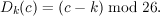
(Notation: x mod 26 is the remainder of x divided by 26.) Thus, if k = 3, then E_k(P) = S and D_k(S) = P .

11.2 Encrypting strings

Of course, one is generally interested in encrypting more than single letter messages, so we need a way to extend the encryption and decryption functions to strings of letters. The simplest way of extending is to encrypt each letter separately using the same key k. If m₁…m_r is an r-letter message, then its encryption is c₁…c_r, where c_i = E_k(m_i) = (m_i + k) mod 26 for each i = 1,…,r. Decryption works similarly, letter by letter.

What we have really done by the above is to build a new cryptosystem from the base cryptosystem on single letters. In the new system, the message space and ciphertext space are

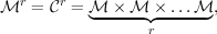
that is, length-r sequences of numbers from {0,…,25}. The encryption and decryption functions are

Here, we use the superscript r to distinguish these functions from the base functions E_k() and D_k().

12 Probabilistic analysis of a simplified Caesar cipher

To make the ideas from Section 11 concrete, we work through a probabilistic analysis of a simplified version of the Caesar cipher restricted to a 3-letter alphabet, so = = = {0,1,2}, E_k(m) = (m + k) mod 3, and D_k(m) = (m - k) mod 3.

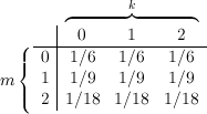
Assume for starters that the message distribution is given in Figure 12.1.

Figure 12.1: A priori message probabilities.

Because the keys are always chosen uniformly, each key has probability 1/3. Hence, we obtain the joint probability distribution shown in Figure 12.2.

Figure 12.2: Joint probability distribution.

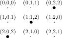
Next, we calculate the conditional probability distribution prob[m = 1∣c = 2]. To do this, we consider the pairs (m,k) in our joint sample space and compute c = E_k(m) for each. Figure 12.3 shows the result, where each point is labeled by a triple (m,k,c), and those points for which c = 2 are shown in bold.

Figure 12.3: Sample space.

The probability that c = 2 is the sum of the probabilities that correspond to the bold face points, i.e., prob[c = 2] = 1∕6 + 1∕9 + 1∕18 = 6∕18 = 1∕3. The only one of these points for which m = 1 is (1,1,2), and it’s probability is 1∕9, so prob[m = 1 ∧ c = 2] = 1∕9. Hence,

Hence, our simplified Caesar cipher is information-theoretically secure.

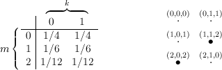
Now let’s make a minor change in the cipher and see what happens. The only change is that we reduce the key space to = {0,1}. The a priori message distribution is still given by Figure 12.1, but the joint probability distribution changes as does the sample space as shown in Figure 12.4.

Figure 12.4: Joint probability distribution and sample space when = {0,1}.

Now, prob[c = 2] = 1∕6 + 1∕12 = 3∕12 = 1∕4, and prob[m = 1 ∧ c = 2] = 1∕6. Hence,

While the a priori probability that m = 1 is still the same as it was before—1/3, the conditional probability given c = 2 is now double what it was. Indeed, there are now only two possibilities for m once Eve sees c = 2. Either m = 1 (and k = 1) or m = 2 (and k = 0). It is no longer possible that m = 0 given that c = 2. Hence, Eve narrows the possibilities for m to the set {1,2}, and her probabilistic knowledge of m changes from the initial distribution (1∕2,1∕3,1∕6) to the new distribution (2∕3,1∕3). She has learned at lot about m indeed, even without finding it exactly!