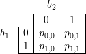
![prob[A (b1,...,bi-1) = bi] ≥ 1+ ϵ
2](ln230x.png)
YALE UNIVERSITY
DEPARTMENT OF COMPUTER SCIENCE
| CPSC 467a: Cryptography and Computer Security | Notes 23 (rev. 1) | |
| Professor M. J. Fischer | December 3, 2008 | |
Lecture Notes 23
One important property of the uniform distribution U on bit-strings b1,…,bℓ is that the individual bits are statistically independent from each other. This means that the probability that a particular bit bi = 1 is unaffected by the values of the other bits in the sequence. Thus, any algorithm that attempts to predict bi, even knowing other bits of the sequence, will be correct only 1/2 of the time. We now translate this property of unpredictability to pseudorandom sequences.
One property we would like a pseudorandom sequence to have is that it be difficult to predict the next bit given the bits that came before.
We say that an algorithm A is an ϵ-next-bit predictor for bit i of a PRSG G if
where (b1,…,bi) = Gi(S). To explain this notation, S is a uniformly distributed random variable ranging over the possible seeds for G. G(S) is a random variable (i.e., probability distribution) over the output strings of G, and Gi(S) is the corresponding probability distribution on the length-i prefixes of G(S).
Next-bit prediction is closely related to indistinguishability, introduced in section 104. We will show later that if if G(S) has a next-bit predictor for some bit i, then G(S) is distinguishable from the uniform distribution U on the same length strings, and conversely, if G(S) is distinguishable from U, then there is a next-bit predictor for some bit i of G(S). The precise definitions under which this theorem is true are subtle, for one must quantify both the amount of time the judge and next-bit predictor algorithms are permitted to run as well as how much better than chance the judgments or predictions must be in order to be considered a successful judge or next-bit predictor. We defer the mathematics for now and focus instead on the intuitive concepts that underlie this theorem.
Suppose a PRSG G has an ϵ-next-bit predictor A for some bit i. Here’s how to build a judge J that distinguishes G(S) from U. The judge J, given a sample string drawn from either G(S) or from U, runs algorithm A to guess bit bi from bits b1,…,bi-1. If the guess agrees with the real bi, then J outputs 1 (meaning that he guesses the sequence came from G(S)). Otherwise, J outputs 0. For sequences drawn from G(S), J will output 1 with the same probability that A successfully predicts bit bi, which is at least 1∕2 + ϵ. For sequences drawn from U, the judge will output 1 with probability exactly 1/2. Hence, the judge distinguishes G(S) from U with advantage ϵ.
It follows that no cryptographically strong PRSG can have an ϵ-next-bit predictor. In other words, no algorithm that attempts to predict the next bit can have more than a “small” advantage ϵ over chance.
Previous-bit prediction, while perhaps less natural, is analogous to next-bit prediction. An ϵ-previous-bit predictor for bit i is an algorithm that, given bits bi+1,…,bℓ, correctly predicts bi with probability at least 1∕2 + ϵ.
As with next-bit predictors, it is the case that if G(S) has a previous-bit predictor for some bit bj, then some judge distinguishes G(S) from U. Again, I am being vague with the exact conditions under which this is true. The somewhat surprising fact follows that G(S) has an ϵ-next-bit predictor for some bit i if and only if it has an ϵ′-previous-bit predictor for some bit j (where ϵ and ϵ′ are related but not necessarily equal).
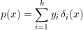
To give some intuition into why such a fact might be true, we look at the special case of ℓ = 2, that is, of 2-bit sequences. The probability distribution G(S) can be described by four probabilities
![p = prob[b = u∧ b = v], where u, v ∈ {0,1}.
u,v 1 2](ln231x.png)
Written in tabular form, we have
We describe an algorithm A(v) for predicting b1 given b2 = v. A(v) predicts b1 = 0 if p0,v > p1,v, and it predicts b1 = 1 if p0,v ≤ p1,v. In other words, the algorithm chooses the value for b1 that is most likely given that b2 = v. Let a(v) be the value predicted by A(v).
Theorem 1 If A is an ϵ-previous-bit predictor for b1, then A is an ϵ-next-bit predictor for either b1 or b2.
Proof: Assume A is an ϵ-previous-bit predictor for b1. Then A correctly predicts b1 given b2 with probability at least 1∕2 + ϵ. We show that A is an ϵ-next-bit predictor for either b1 or b2.
We have two cases:
Case 1: a(0) = a(1). Then algorithm A does not depend on v, so A itself is also an ϵ-next-bit predictor for b1.
Case 2: a(0)≠a(1). The probability that A(v) correctly predicts b1 when b2 = v is given by the conditional probability
![prob[b = a(v) | b = v ] = prob[b1 =-a(v)-∧b2-=-v]=--pa(v),v---
1 2 prob[b2 = v] prob[b2 = v]](ln233x.png)
The overall probability that A(b2) is correct for b1 is the weighted average of the conditional probabilities for v = 0 and v = 1, weighted by the probability that b2 = v. Thus,
![prob[A(b2) is correct for b1] = ∑ prob[b1 = a(v) | b2 = v]⋅prob[b2 = v ]
v∈{0,1}
∑
= pa(v),v
v∈{0,1}
= pa(0),0 + pa(1),1](ln234x.png)
Now, since a(0)≠a(1), the function a is one-to-one and onto. A simple case analysis shows that either
a(v) = v for v  {0,1}, or a(v) = ¬v for v {0,1}. That is, a is either the identity or the complement
function. In either case, a is its own inverse. Hence, we may also use algorithm A(u) as a predictor for b2
given b1 = u. By a similar analysis to that used above, we get
{0,1}, or a(v) = ¬v for v {0,1}. That is, a is either the identity or the complement
function. In either case, a is its own inverse. Hence, we may also use algorithm A(u) as a predictor for b2
given b1 = u. By a similar analysis to that used above, we get
![∑
prob[A (b1) is correct for b2] = prob[b2 = a(u) | b1 = u]⋅prob[b1 = u]
v∈∑{0,1}
= pu,a(u)
v∈{0,1}
= p + p
0,a(0) 1,a(1)](ln235x.png)

since either a is the identity function or the complement function. Hence, A(b1) is correct for b2 with the same probability that A(b2) is correct for b1. Therefore, A is an ϵ-next-bit predictor for b2.
In both cases, we conclude that A is an ϵ-next-bit predictor for either b1 or b2. __
There are many situations in which one wants to grant access to a resource only if a sufficiently large group of agents cooperate. For example, a store safe might require both the manager’s key and the armored car driver’s key in order to be opened. This protects the store against a dishonest manager or armored car driver, and it also prevents an armed robber from coercing the manager into opening the safe. A similar 2-key system is used for safe deposit boxes in banks.
We might like to achieve the same properties for cryptographic keys or other secrets. For example, if k is the secret decryption key for a cryptosystem, one might wish to split k into two shares k1 and k2. By themselves, neither k1 nor k2 reveals any information about k, but when suitably combined, k can be recovered. A simple way to do this is to choose k1 uniformly at random and then let k2 = k ⊕ k1. Both k1 and k2 are uniformly distributed over the key space and hence give no information about k. However, combined with XOR, they reveal k, since k = k1 ⊕ k2.
Indeed, the one-time pad cryptosystem of lecture notes 3, section 14, can be viewed as an instance of secret splitting. Here, Alice’s secret is her message m. The two shares are the ciphertext c and the key k. Neither by themselves gives any information about m, but together they reveal m = k ⊕ c.
Secret splitting generalizes to more than two shares. Imagine a large company that restricts access to important company secrets to only its five top executives, say the president, vice-president, treasurer, CEO, and CIO. They don’t want any executive to be able to access the data alone since they are concerned that an executive might be blackmailed into giving confidential data to a competitor. On the other hand, they also don’t want to require that all five executives get together to access their data, both because this would be cumbersome and also because they worry about the death or incapacitation of any single individual. They decide as a compromise that any three of them should be able to access the secret data, but not one or two of them operating alone.
A (τ,k) threshold secret splitting scheme splits a secret s into shares s1,…,sk. Any subset of τ or more shares allows s to be recovered, but no subset of shares of size less than τ gives any information about s.
Shamir proposed a threshold scheme based on polynomials. A polynomial of degree d is an expression
 | (1) |
where ad≠0. The numbers a0,…,ad are called the coefficients of f. A polynomial can be simultaneously regarded as a function and as an object determined by its vector of coefficients.
Interpolation is the process of finding a polynomial that goes through a given set of points. Fact Let (x1,y1),…,(xk,yk) be points, where all of the xi’s are distinct. There is a unique polynomial f(x) of degree at most k - 1 that passes through all k points, that is, for which f(xi) = yi (1 ≤ 1 ≤ k).
f can be found using Lagrangian interpolation. This statement generalizes the familiar statement from high school geometry that two points determine a line.
One way to understand Lagrangian interpolation is to consider the polynomial

Although this looks at first like a rational function, it is actually just a polynomial in x since the denominator contains only the x-values of the given points and not the variable x. δi(x) has the easily-checked property that δi(xi) = 1, and δi(xj) = 0 for j≠i. Then the polynomial
is the desired interpolating polynomial, since p(xi) = yi for i = 1,…,k. Note that to actually find the coefficients of p(x) when written in the canonical form of equation 1, it is necessary to expand p(x) by multiplying out the factors and collecting like terms.
Interpolation also works over finite fields, for example, Zp for prime p. That is, any k points with distinct x coordinates determine a unique polynomial of degree at most k - 1 over Zp. Of course, we must have k ≤ p since Zp has only p distinct coordinate values in all.
Here’s how Shamir’s (τ,k) secret splitting scheme works. Let Alice (also called the dealer) have
secret s. She constructs a polynomial of degree at most τ - 1 as follows: She sets a0 = s,
and she chooses a1,…,aτ-1 Zp at random. Share si is the point (xi,yi), where xi = i and
yi = f(i)(1 ≤ i ≤ k)1 .
Theorem 2 s can be reconstructed from any set T of τ or more shares.
Theorem 3 Any set T′ of fewer than τ shares gives no information about s.
Zp, there is a polynomial
gs′ that interpolates the shares in T′∪{(0,s′)}. Each of these polynomials passes through all of the
shares in T′, so each is a plausible candidate for f. Moreover, gs′(0) = s′, so each s′ is a plausible
candidate for the secret s. One can show further that the number of polynomials that interpolate
T′∪{(0,s′)} is the same for each s′ Zp, so each possible candidate s′ is equally likely to be s.
Hence, the shares in T′ give no information at all about s. __
Several variations on secret sharing have been studied. I mention two briefly but do not go into details.
A dealer has a secret s which she wishes to share with a number of players. The dealer can of course always lie about the true value of her secret, but, as with bit commitment, the players want assurance that their shares do in fact code a unique secret. That is, whenever sufficiently many shares are assembled to reconstruct the secret, the same secret s is recovered, no matter which shares are used. In Shamir’s (τ,k) threshold scheme, this will be true only if all of the shares lie on a single polynomial of degree at most k - 1. However, if the dealer is dishonest and gives bad shares to some of the players, the resulting shares might not lie on any polynomial of degree k - 1 or smaller. The players have no way to discover this until later when they try to reconstruct s.
In verifiable secret sharing, the sharing phase is an active protocol involving the dealer and all of the players. At the end of this phase, either the dealer is exposed as being dishonest, or all of the players end up with shares that are consistent with a single secret. Needless to say, protocols for verifiable secret sharing are quite complicated.
Even if the dealer is assumed to be honest, there is still the problem of actively dishonest players. With Shamir’s scheme, a share that just disappears does not prevent the secret from being reconstructed, as long as enough valid shares remain. But if a player lies about his share and presents a corrupted share, then that share might be used by the other players in reconstructing an incorrect value for the secret. A fault-tolerant secret sharing scheme should allow the secret to be correctly reconstructed, even in the face of a certain number of corrupted shares.
Of course, it may be desirable to have schemes that can tolerate dishonesty in both dealer and a certain number of players. The interested reader is encouraged to explore the extensive literature on this subject.
Alice and Bob want to play a game over the internet. Alice says, “I’m thinking of a bit. If you guess my bit correctly, I’ll give you $10. If you guess wrong, you give me $10.” Bob says, “Ok, I guess zero.” Alice replies, “Sorry, you lose. I was thinking of one.”
While this game may seem fair on the surface, there is nothing to prevent Alice from changing her mind after Bob makes his guess. Even if Alice and Bob play the game face to face, they still must do something to commit Alice to her bit before Bob makes his guess. For example, Alice might be required to write her bit down on a piece of paper and seal it in an envelope. After Bob makes his guess, he opens the envelope and knows whether he has won or lost. The act of writing down the bit commits Alice to that bit, even though Bob doesn’t learn its value until later.
The bit commitment problem is to implement an electronic form of sealed envelope called a commitment or blob or cryptographic envelope. Intuitively, a blob has two properties: (1) It is not possible to see the bit inside the blob without opening it. (2) It is not possible to change the bit inside the blob, that is, the blob cannot be opened in two different ways to reveal two different bits.
A blob is produced by a protocol commit(b) between Alice and Bob. We assume that b is initially private to Alice. At the end of the commit protocol, Bob has a blob c containing Alice’s bit b, but he should have no information about b’s value. Later, Alice and Bob can run a protocol open(c) to reveal the bit contained in c.
Alice and Bob do not trust each other, so each wants protection from cheating by the other. Alice wants to be sure that Bob cannot learn b after running commit(b), even if he misbehaves during the protocol. Bob wants to be sure that any successful run of open(c) reveals the same bit b′, so no matter what Alice does. Note that we do not require that Alice tell the truth about her private bit b. A dishonest Alice can always pretend her bit was b′≠b when producing c. But if she does, c can only be opened to b′, not to b.
These ideas should become clearer in the protocols below.
A naïve way to use a symmetric cryptosystem for bit commitment is for Alice to commit b by encrypting it with a private key k to get a blob c = Ek(b). She later opens it using the decryption function Dk(c). Unfortunately, Alice can easily cheat if she can find a “colliding triple” (c,k0,k1) with the properties that Dk0(c) = 0 and Dk0(c) = 1. She just “commits” by sending c to Bob. Later, she can choose whether to open it to 0 or to 1 by sending Bob k0 or k1. This isn’t just a hypothetical problem. Suppose Alice uses the most secure cryptosystem of all, a one-time pad (lecture notes 3, section 14), so Dk(c) = c ⊕ k. Then she can easily find a colliding triple by choosing k0 = c and k1 = c ⊕ 1.
The protocol of Figure 113.1 tries to make it harder for Alice to cheat by making it possible for Bob to detect most bad keys.
For many cryptosystems (e.g., DES), this protocol does indeed prevent Alice from cheating, for she will
have difficulty finding any two keys k0 and k1 such that Ek0(r ⋅ 0) = Ek1(r ⋅ 1). However, for the one-time
pad cryptosystem, she can cheat as before: She just takes c to be random and lets k0 = c ⊕ (r ⋅ 0) and
k1 = c ⊕ (r ⋅ 1). Then Dkb(c) = r ⋅ b for b {0,1}, so the revealed bit is 0 or 1 depending on whether
Alice sends k0 or k1 in step 3.
We see that not all secure cryptosystems have the properties we need in order to make the protocol of Figure 113.1 secure. We need a property analogous to the strong collision-free property for hash functions (lecture notes 14, section 78).
 .
. 
